Analysing the effect of bog ditches on Sphagnum communities

1 Introduction

This web page documents the preparation of a data set on the effects of hydrological disturbance on the growth of Sphagnum mosses on a Norwegian bog, before uploading it to GBIF.

After this initial introduction chapter, (data-exp?) goes through the data cleaning and general formatting, and (mapping?) describes how individual columns in the spreadsheet have been mapped to DwC terms.

The raw datafiles are found under data/and has not been altered. Instead, all data manipulation (formatting, fixing typos, adding metadata etc.) has been scripted and is presented in this work.

The data collection was done by employees at the NTNU University Museum during the years 2017-2022. Part of the motivation for this work was to get baseline data before a planned mire resturation project. The mire resturation has not been realised. However, the data also serves as a valuabla dataset for environmental gradient analyses of Sphagnum communities.

Figure 1.1 shows a map of the bog, which is a relatively large ombrotrophic bog previously used for peat extraction, and also drained and used for forest plantations. Sphagnum growth was measured using the cranked wire technique on permanent vegetation quadrats (n = 28) from 2017 to 2022 (5 growing seasons). Each vegetation quadrat has 16 points (i.e. pins) and each pin was measured up to 4 times on each sampling occasion (on each side and by different people). The first 18 vegetation plots were initiated in 2017 and are paired with water table well that log the water table depth. These vegetation plots are situated in homogeneous vegetation types (bog lawns), but with varying distance to disturbances (extraction sites and ditches). The quadrats numbered 18-28 were initiated in 2021 and a placed relatively for from the hydrological disturbances, but in varying communities (hollows and hummoks).

library(tidyverse)
library(sf)
library(tmap)

path    <- "data/shapeFiles/"
ditches <- sf::read_sf(paste0(path, "ditches/grofter.shp"))
massifs  <- sf::read_sf(paste0(path, "massifs/hostadmyra_myrmassiv.shp")) 

#extrSites <- sf::read_sf(paste0(path, "peatExtractionSites/Torvtak.shp"))
# This data is the same as the masifs.

quadrats <- sf::read_sf(paste0(path, "vegetationQuadrats1/veipunkter_vannbronner_ruter_2017.shp")) |>
  bind_rows(sf::read_sf(paste0(path, "vegetationQuadrats2/vegetasjonsruter_19-30.shp")))

tm_shape(massifs) +
  tm_polygons(col = "Name",
              palette = c("grey60", "grey70", "grey80"),
              legend.show=F) +
  tm_shape(ditches |>
             mutate("Ditch age" = case_when(
               Name == "Eldre" ~ "Old",
               Name == "Nyere" ~ "More recent",
               .default = "Old"
             ))) +
  tm_lines(col = "Ditch age",
           lwd=2,
           palette = c("red", "orange")) +
  #tm_shape(extrSites) +
  #tm_polygons()
  tm_shape(quadrats) +
  tm_dots(size = 2,
          shape=21,
          col = "green",
          alpha = 0.5)  +
  tm_scale_bar(position = c("left", "bottom")) +
  tm_compass()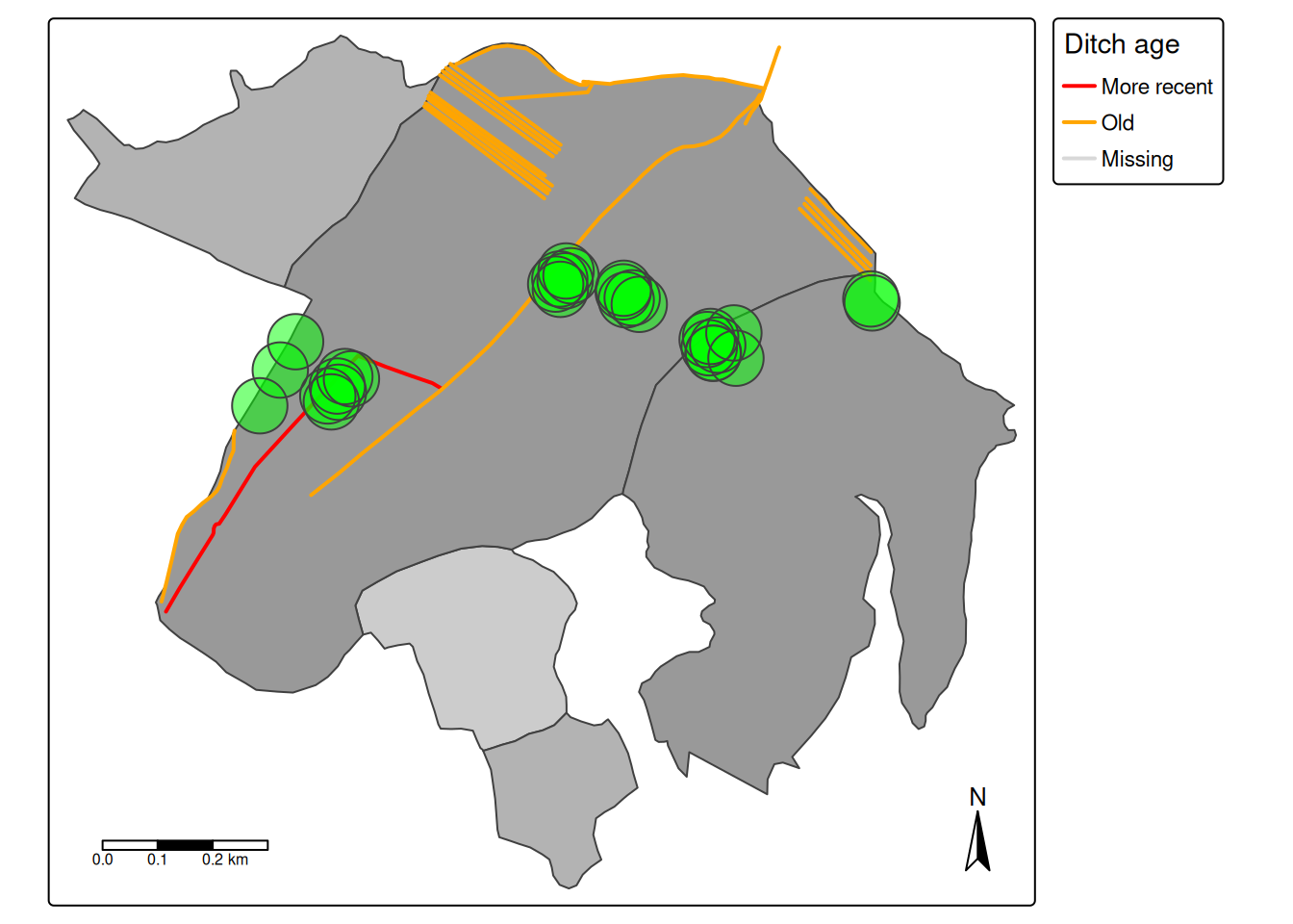

Figure 1.1: Map of study area. Green circles are permanent vegetation quadrats. The shades of grey indicator different bog massifs.

The shape file with the position of vegetation quadrats do not contain the quadrat ID for all cases. We need to add that.