ea_spread
ea_spread.RdA function to aggregate (area weigted means) indicator values stored in a spatial object (sf or stars object) for each homogeneous area class, and subsequently to spread these values out to populate all the area for the homogeneous area classes.
Arguments
- indicator_data
A spatial object (currently inlo sf objects are supported) containing scaled indicator values
- indicator
Column name in
indicator_datacontaining indicator values. Should be unquoted.- regions
An sf object where polygon values (slect which colum using the
groupsargument) assign areas to homogeneous area classes. If you have a raster, useea_homogeneous_areas()to convert it to sf.- groups
Name in
regionscontaining homogeneous area classes. Should be unquoted.- threshold
Number of data points (i.e. unique indicator values) needed to calculate an average indicator value. Defaults to 1 (i.e. no threshold).
- summarise
Logical. Should the function return an sf object with wall-to-wall mean indicator values (default, summarise = FALSE), or should the function return a data frame with summary statistics
Value
In case tally = FALSE, the returned object is an sf object containing homogeneous area classes and wall-to-wall mean indicator values. If tally = TRUE, a data frame with summary statistics is returned. Indicator values are areas weighted (w_mean). If summarise = TRUE, the unweighted mean is also returned (mean), along with the number of data points (n), the total area with indicator data, and the standard deviation. The SD is returned in both cases, and is produced from non-parametric bootstrapping with 1000 replications.
Examples
data("ex_polygons")
data("ex_raster")
# Example using a raster to define homogeneous area classes.
# Zooming in on the example data
ex_raster_zoom <- ex_raster[,5:6, 28:29]
ex_polygons_zoom <- sf::st_crop(ex_polygons, ex_raster_zoom)
#> Warning: attribute variables are assumed to be spatially constant throughout all geometries
# Scale the indicator
ex_polygons_zoom$indicator <- ea_normalise(ex_polygons_zoom,
"condition_variable_2",
upper_reference_level = 7)
# Tweak the data slightly for exaggerated effect
ex_polygons_zoom$indicator[2:6] <- 1
# Process the `ex_raster_zoom` and define homogeneous areas based on the cell values.
myRegions <- ea_homogeneous_area(ex_raster_zoom,
groups = values)
# Now use the function
out <- ea_spread(indicator_data = ex_polygons_zoom,
indicator = indicator,
regions = myRegions,
groups = values)
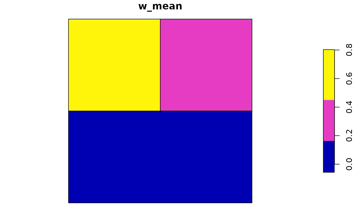
# And plot the results
plot(out[,2])
 # Example 2: Summary output
ea_spread(indicator_data = ex_polygons_zoom,
indicator = indicator,
regions = myRegions,
groups = values,
summarise = TRUE)
#> values total_area n w_mean mean sd
#> 1 1 69675.832 30 0.24102147 0.3708932 0.06772947
#> 2 2 58330.105 7 0.08642357 0.3810810 0.12949363
#> 3 3 3351.623 3 0.65946526 0.7039941 0.21289913
# Example 2: Summary output
ea_spread(indicator_data = ex_polygons_zoom,
indicator = indicator,
regions = myRegions,
groups = values,
summarise = TRUE)
#> values total_area n w_mean mean sd
#> 1 1 69675.832 30 0.24102147 0.3708932 0.06772947
#> 2 2 58330.105 7 0.08642357 0.3810810 0.12949363
#> 3 3 3351.623 3 0.65946526 0.7039941 0.21289913