Aggregate indicators to regions

library(eaTools)
library(tmap)
library(stars)
library(dplyr)
library(stats)
library(ggplot2)

Introduction

We are often in a position where we need to aggregate indicators to certain regions within a larger accounting area. This process is a little different depending on the spatial coverage of the indicator and whether the regions are defined in a raster or with polygons.

We will use some example data sets included in the package.

data("ex_polygons")
data("accounting_area")
data("ex_raster")

tm_shape(ex_raster)+
  tm_raster(alpha = 1,
            style = "cat")+
  tm_shape(accounting_area)+
  tm_polygons(alpha = .6)+
  tm_shape(ex_polygons)+
  tm_polygons(border.col = "black")+
  tm_layout(legend.outside = T)+
  tm_scale_bar(position = c("right", "bottom"), width = 0.3)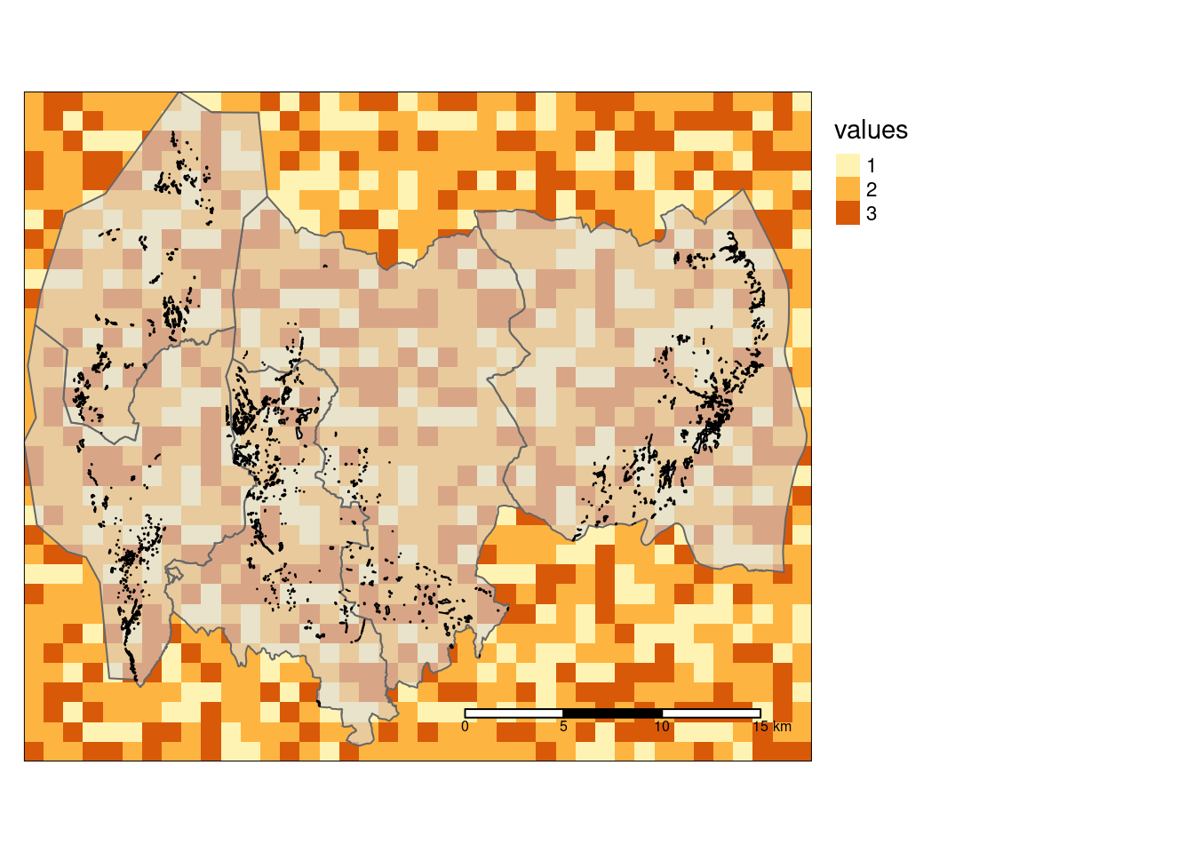

Figure 1: Showing the three example datasets on top of eachother. The raster layer (ex_raster) have cell values 1, 2 or 3, as shown in the legend. The five large polygons is the accounting_area layer, and the smaller polygins, visible as specks, is teh ex_polygons layer.

Case 1: Aggregate indicator values from small polygons for each of the three classes in the raster layer, and spread them to cover the entire raster layer.

In this example we are imagining that ex_polygons, and the column condition_variable_2, contains a condition variable, and that ex_raster denotes homogeneous areas. We aknowledge a spatial bias in the sampling of the dummy condition variable. However, in this hypothetical example, we think that the variable/indicator can be said to be representative of the homogeneous area class that it belongs to. We therefore allow ourselves to extrapolate, or spread, the mean indicator values within a given homogeneous area class to the other grid cells of the same class.

To be able to see what we are doing, we will zoom in on the data above.

ex_raster_zoom <- ex_raster[,5:6, 28:29]
ex_polygons_zoom <- sf::st_crop(ex_polygons, ex_raster_zoom)

First we would scale the variable, and make it into an indicator using ea_normalise() (See vignette("Normalise condition variable")).

ex_polygons_zoom$indicator <- ea_normalise(ex_polygons_zoom,
                                           "condition_variable_2",
                                           upper_reference_level = 7)

ggplot(ex_polygons_zoom, aes(x = indicator))+
  geom_histogram(fill = "grey",
                 colour = "black",
                 size = 1.2)+
  theme_bw(base_size = 12)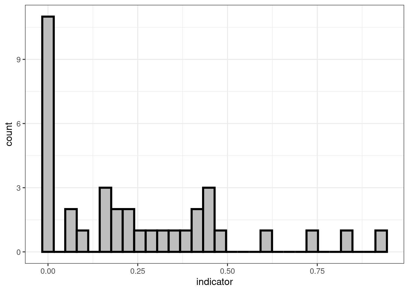

Figure 2: Histogram of the example indicator values.

tm_shape(ex_raster_zoom)+
  tm_raster(style="cat")+
  tm_shape(ex_polygons_zoom)+
  tm_polygons(col = "indicator",
              palette = "RdYlGn",
              border.col = "black")+
  tm_layout(legend.outside = T)+
  tm_scale_bar(position = c("left", "bottom"), width = 0.3)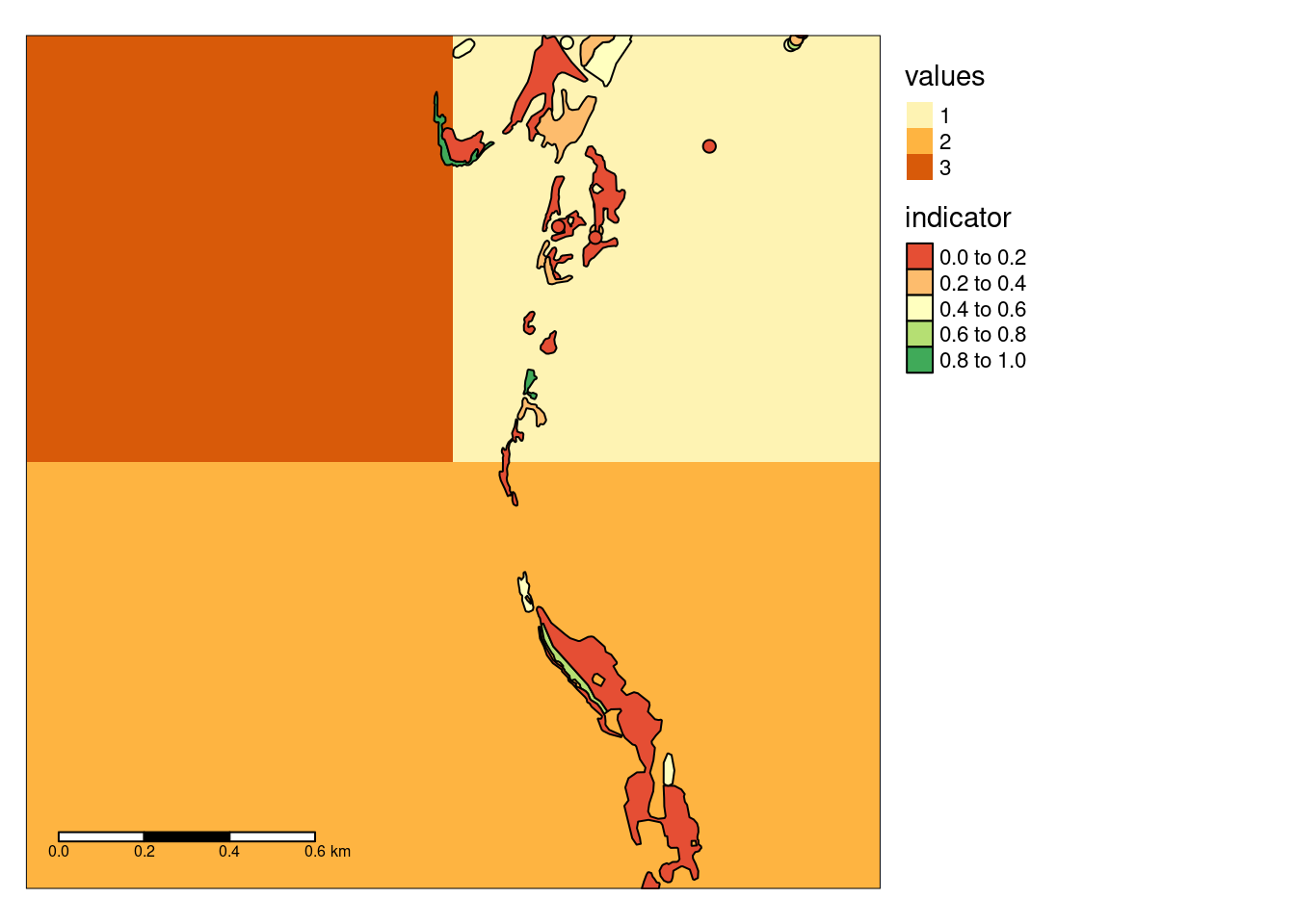

Figure 3: Example data produced by zooming in on four grid cells in the above figure.

I will manipulate the data set slightly, just to make some contrasts between the three homogeneous area classes more visible.

ex_polygons_zoom$indicator[2:6] <- 1

We now want to calculate the area weighted mean for each homogeneous area class, i.e. the three different colored grid cells in Fig. 3.

First we process ex_raster_zoom (vectorise it) and define homogeneous areas based on the cell values.

myRegions <- ea_homogeneous_area(ex_raster_zoom,
                                 groups = values)

Then we aggregate the indicator values from ex_polygons_zoom for each homogeneous area class, and spread the mean indicator values across all the grid cells. Even grid cells that originally had no indicator values associated with it will be populated with the area weighted mean of its homogeneous area class. Lets to this step with and without defining a threshold for how many data points we need before calculating an average.

myIndicator <- ea_spread(indicator_data = ex_polygons_zoom,
                         indicator = indicator,
                         regions = myRegions,
                         groups = values,
                         threshold = 5)

myIndicator_noThreshold <- ea_spread(indicator_data = ex_polygons_zoom,
                         indicator = indicator,
                         regions = myRegions,
                         groups = values)

tmap_arrange(
  
  # W/ threshold
  tm_shape(myIndicator)+
    tm_polygons(col = "w_mean",
                title="Indicator value",
                palette = "RdYlGn",
                breaks = seq(0,1,0.2))+
    tm_shape(ex_polygons_zoom)+
    tm_polygons(col = "indicator",
                legend.show = F,
                palette = "RdYlGn",
                breaks = seq(0,1,0.2),
                border.col = "black")+
    tm_layout(legend.position = c('left', 'top'),
              title = "Threshold = 5 data points"),
  
  
  # No threshold
  tm_shape(myIndicator_noThreshold)+
    tm_polygons(col = "w_mean",
                title="Indicator value",
                palette = "RdYlGn",
                breaks = seq(0,1,0.2))+
    tm_shape(ex_polygons_zoom)+
    tm_polygons(col = "indicator",
                legend.show = F,
                palette = "RdYlGn",
                breaks = seq(0,1,0.2),
                border.col = "black")+
    tm_layout(legend.position = c('left', 'top'),
              title = "No threshold"),
  
  # errors 
  tm_shape(myIndicator)+
    tm_polygons(col = "sd",
                title="Standard error",
                palette = "-RdYlGn",
                n=4)+
    tm_layout(legend.position = c('left', 'top')),
  # errors
  tm_shape(myIndicator_noThreshold)+
    tm_polygons(col = "sd",
                title="Standard error",
                palette = "-RdYlGn",
                n=4)+
    tm_layout(legend.position = c('left', 'top')),
  heights = c(.8,.2)
)

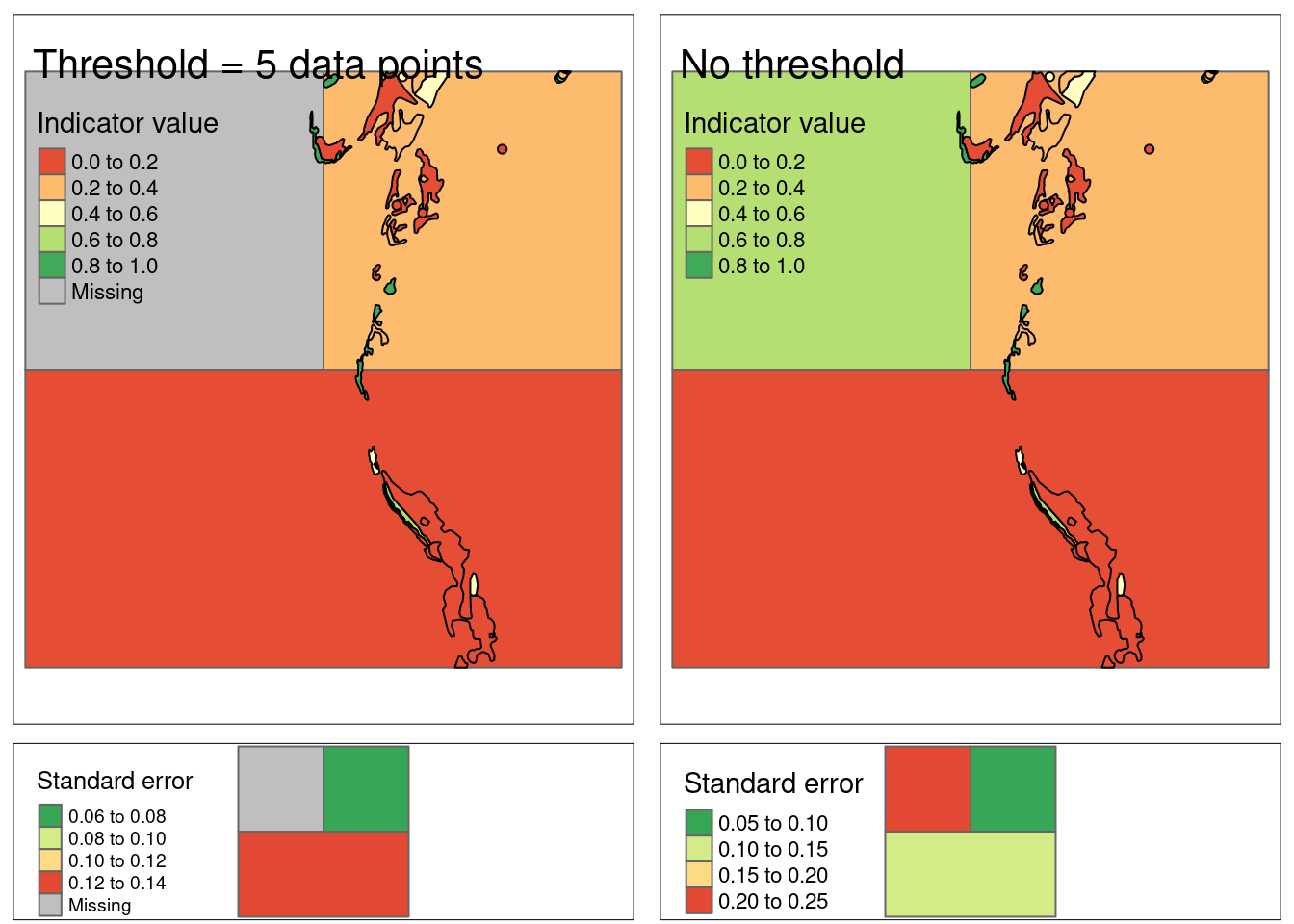
Figure 4: Example where the area weighted averages of the indicator values in the small polygons are spread over the raster cells with each homogeneous area class. In the left example, only homogeneous area class with more than 5 data points get indicator values. The standard errors for the extrapolated indicator values is shown in the bottom row, and are produced by bootstrapping the indicator data in the small polygoins.

In the map above (the top row), the color of the cells are in a way the average color of the polygons that overlay these cells. Note that the bottom left cell (still in the top row) now still has an indicator value even though it didn’t have any data to start with.

If we look at the top right figure, homogeneous area class 3 (top left cell) is in better condition, but this indicator value is based on very few data points (3 in fact, as you can see in th next table). If we assign a threshold above the number of available data points, the function returns NA (right column). The low number of data points for homogeneous area class 3 is also reflected in the large standard deviatio for that estimate (bottom right pane).

We can also use the same function to return the values, including some summary statistics, as a data frame:

ea_spread(indicator_data = ex_polygons_zoom,
                         indicator = indicator,
                         regions = myRegions,
                         groups = values,
                         summarise = T)
#>   values total_area  n     w_mean      mean         sd
#> 1      1  69675.832 30 0.24102147 0.3708932 0.06574245
#> 2      2  58330.105  7 0.08642357 0.3810810 0.12490779
#> 3      3   3351.623  3 0.65946526 0.7039941 0.22019339

We can then chose rasterise this back again, because a raster format is more useful for subsequent analyses, such as aggregating indicators. Here we can use an existing function from the sf package.

newIndicator_raster <- stars::st_rasterize(myIndicator, ex_raster_zoom)