Binarize continuous raster maps

Through GRASS GIS, this function transforms continuous or categorical maps (with more than 1 category) into binary maps (with only two values), to represent, e.g., habitat-matrix maps in the context of landscape ecology. It can also be used to produce binary maps form maps with only one category (and all the rest as NULL/no-data). It requires an active connection between the R session and a GRASS GIS location and mapset (through the package rgrass), and that the input map is already loaded within this GRASS GIS mapset.

Usage

grass_binarize(
  x,
  breaks = 0.5,
  output = paste0(x, "_bin"),
  null = NULL,
  setnull = NULL,
  bin_values = c(0, 1),
  input_as_region = FALSE,
  verbose = FALSE,
  overwrite = FALSE,
  ...
)

Arguments

x: [character(1)]
Name of the input raster map, within a GRASS GIS location and mapset.
breaks: [numeric]
Breaks or threshold to define the binary values in the output binary map. All pixels with value >= breaks are considered as 1 (or the upper value defined in bin_values), and all the rest are considered as 0 (or the lower value defined in bin_values). breaks might be either a single numeric value or a vector of numeric values, in which case multiple binary maps are created (with different break thresholds).
output: [character(1)]
Name of the output map, or prefix of the output map if length(breaks) > 1. In the latter case, the names are completed with the break value. The defult is to use the same name as the input map, plus "_bin" in the end.
null: [numeric(1)=NULL]
If NULL (default), all NULL/no-data pixels in from x are kept as they are in the output map. Otherwise, a numeric value that all NULL pixels should assume in the output map. It uses the module r.null).
setnull: []
If NULL (default), no changes are made. Otherwise, a set of numeric values that should be transformed into NULL/NA data (using the module r.null).
bin_values: [numeric(2)=c(0,1)]
Values c(lower, upper) that the output map pixels should have if their values are either "lower" or "equal or higher" breaks. By default, c(0, 1).
input_as_region: [logical(1)=FALSE]
Should the input map x be used to redefine the working region in GRASS before raster binarization? If TRUE, x is used to define the region with g.region. If FALSE, the region previously defined in the GRASS GIS session is used for computation. Default is FALSE.
verbose: [logical(1)=FALSE]
Should messages of the computation steps be printed in the prompt along the computation?
overwrite: [logical(1)]
Whether the output maps should be overwriten (flag overwrite = TRUE).

Value

A binarized map with only two values (or a set of binarized maps if length(breaks) > 1) within the GRASS GIS mapset. In R, the output is a string with the name of this map.

Details

For a similar procedure within R, use raster algebra functions within the raster and terra packages.

Examples

# libraries
library(rgrass)
library(terra)

# Load raster data
f <- system.file("raster/sample_area_cabins.tif", package = "oneimpact")
cabins <- terra::rast(f)

# connect to grass gis and create grass location
# For linux or within OSGeo4W shell
grassdir <- system("grass --config path", intern = TRUE)
# grassdir <- system("grass78 --config path", intern = TRUE) # for GRASS 7.8
# If you used the standalone installer in Windows
# grassdir <- "C:\Programs\GRASS GIS 7.8" # Correct if the path GRASS version or path is different

gisDB <- "." # create location and mapset in the working directory
loc <- "ETRS_33N/" # name of the location
ms <- "PERMANENT" # name of the mapset
rgrass::initGRASS(gisBase = grassdir,
                  SG = cabins, # use map to define location projection
                  home = tempdir(),
                  override = TRUE,
                  gisDbase = gisDB,
                  location = loc,
                  mapset = ms)
#> gisdbase    . 
#> location    ETRS_33N/ 
#> mapset      PERMANENT 
#> rows        361 
#> columns     478 
#> north       6658900 
#> south       6622800 
#> west        146900 
#> east        194700 
#> nsres       100 
#> ewres       100 
#> projection:
#>  PROJCRS["unknown",
#>     BASEGEOGCRS["grs80",
#>         DATUM["European Terrestrial Reference System 1989",
#>             ELLIPSOID["Geodetic_Reference_System_1980",6378137,298.257222101,
#>                 LENGTHUNIT["metre",1]],
#>             ID["EPSG",6258]],
#>         PRIMEM["Greenwich",0,
#>             ANGLEUNIT["degree",0.0174532925199433,
#>                 ID["EPSG",9122]]]],
#>     CONVERSION["Transverse Mercator",
#>         METHOD["Transverse Mercator",
#>             ID["EPSG",9807]],
#>         PARAMETER["Latitude of natural origin",0,
#>             ANGLEUNIT["degree",0.0174532925199433],
#>             ID["EPSG",8801]],
#>         PARAMETER["Longitude of natural origin",15,
#>             ANGLEUNIT["degree",0.0174532925199433],
#>             ID["EPSG",8802]],
#>         PARAMETER["Scale factor at natural origin",0.9996,
#>             SCALEUNIT["unity",1],
#>             ID["EPSG",8805]],
#>         PARAMETER["False easting",500000,
#>             LENGTHUNIT["metre",1],
#>             ID["EPSG",8806]],
#>         PARAMETER["False northing",0,
#>             LENGTHUNIT["metre",1],
#>             ID["EPSG",8807]]],
#>     CS[Cartesian,2],
#>         AXIS["easting",east,
#>             ORDER[1],
#>             LENGTHUNIT["metre",1,
#>                 ID["EPSG",9001]]],
#>         AXIS["northing",north,
#>             ORDER[2],
#>             LENGTHUNIT["metre",1,
#>                 ID["EPSG",9001]]]] 

# add map to GRASS
rgrass::write_RAST(cabins, "cabins", flags = "o")
#> Over-riding projection check
#> Importing raster map <cabins>...
#>    0%   3%   6%   9%  12%  15%  18%  21%  24%  27%  30%  33%  36%  39%  42%  45%  48%  51%  54%  57%  60%  63%  66%  69%  72%  75%  78%  81%  84%  87%  90%  93%  96%  99% 100%
#> SpatRaster read into GRASS using r.in.gdal from file

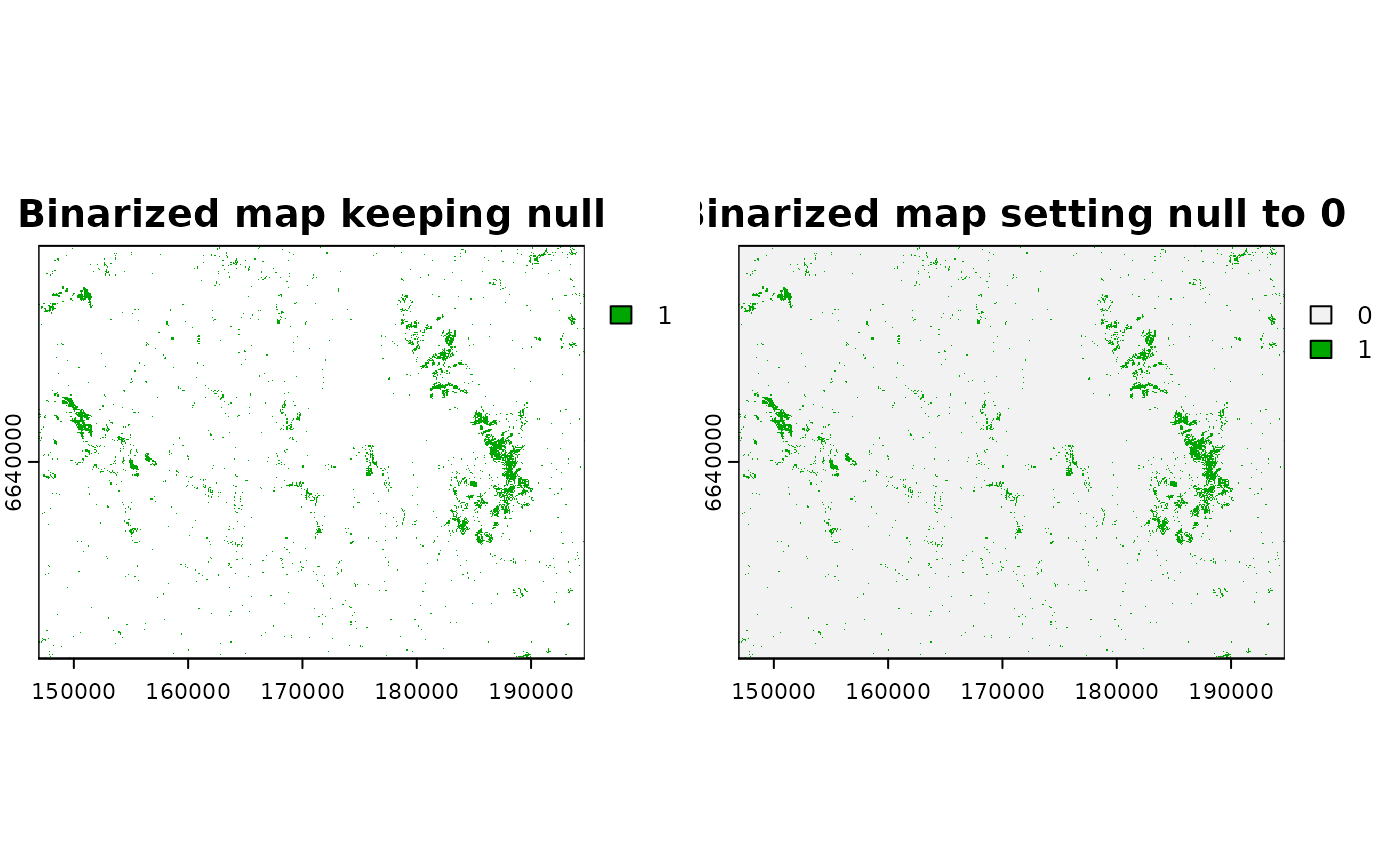
# binarize the input map

# map with only 1
cabins_bin1_name <- grass_binarize("cabins", output = "cabins_bin1",
                                   breaks = 1, overwrite = T)
# map with 0, 1
cabins_bin2_name <- grass_binarize("cabins", output = "cabins_bin2",
                                   breaks = 1, null = 0, overwrite = T)
#> Removing raster <inter_map>

# visualize
cabins_bin1_2 <- rgrass::read_RAST(c(cabins_bin1_name, cabins_bin2_name),
                                   return_format = "terra", NODATA = 255)
#> Checking GDAL data type and nodata value...
#>    2%   5%   8%  11%  14%  17%  20%  23%  26%  29%  32%  35%  38%  41%  44%  47%  50%  53%  56%  59%  62%  65%  68%  71%  74%  77%  80%  83%  86%  89%  92%  95%  98% 100%
#> Using GDAL data type <Byte>
#> Exporting raster data to RRASTER format...
#>    2%   5%   8%  11%  14%  17%  20%  23%  26%  29%  32%  35%  38%  41%  44%  47%  50%  53%  56%  59%  62%  65%  68%  71%  74%  77%  80%  83%  86%  89%  92%  95%  98% 100%
#> r.out.gdal complete. File </tmp/RtmpXUdBg8/file26cb19face30.grd> created.
#> Checking GDAL data type and nodata value...
#>    2%   5%   8%  11%  14%  17%  20%  23%  26%  29%  32%  35%  38%  41%  44%  47%  50%  53%  56%  59%  62%  65%  68%  71%  74%  77%  80%  83%  86%  89%  92%  95%  98% 100%
#> Using GDAL data type <Byte>
#> Exporting raster data to RRASTER format...
#>    2%   5%   8%  11%  14%  17%  20%  23%  26%  29%  32%  35%  38%  41%  44%  47%  50%  53%  56%  59%  62%  65%  68%  71%  74%  77%  80%  83%  86%  89%  92%  95%  98% 100%
#> r.out.gdal complete. File </tmp/RtmpXUdBg8/file26cb6ede5390.grd> created.
plot(cabins_bin1_2, main = c("Binarized map keeping null", "Binarized map setting null to 0"))


#-------
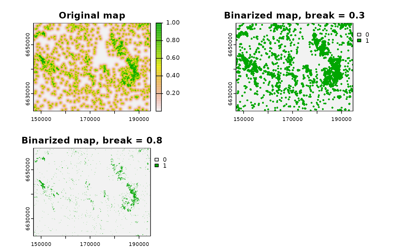
# binarize the map with multiple break values

# first create a continuous map
cont_map_name <- calc_zoi_nearest("cabins_bin1", radius = 1000,
                                  type = "exp_decay",
                                  where = "GRASS", overwrite = TRUE)
#> Removing raster <cabins_bin1_zoi_nearest_euclidean>
# binarize
cabins_bin2vals_name <- grass_binarize(cont_map_name, output = "cabins_zoi1000_bin",
                                       breaks = c(0.3, 0.8), overwrite = T)
# visualize
cabins_bin2vals <- rgrass::read_RAST(c(cont_map_name, cabins_bin2vals_name),
                                     return_format = "terra", NODATA = 255)
#> Checking GDAL data type and nodata value...
#>    2%   5%   8%  11%  14%  17%  20%  23%  26%  29%  32%  35%  38%  41%  44%  47%  50%  53%  56%  59%  62%  65%  68%  71%  74%  77%  80%  83%  86%  89%  92%  95%  98% 100%
#> Using GDAL data type <Float64>
#> Exporting raster data to RRASTER format...
#>    2%   5%   8%  11%  14%  17%  20%  23%  26%  29%  32%  35%  38%  41%  44%  47%  50%  53%  56%  59%  62%  65%  68%  71%  74%  77%  80%  83%  86%  89%  92%  95%  98% 100%
#> r.out.gdal complete. File </tmp/RtmpXUdBg8/file26cb3ac541ac.grd> created.
#> Checking GDAL data type and nodata value...
#>    2%   5%   8%  11%  14%  17%  20%  23%  26%  29%  32%  35%  38%  41%  44%  47%  50%  53%  56%  59%  62%  65%  68%  71%  74%  77%  80%  83%  86%  89%  92%  95%  98% 100%
#> Using GDAL data type <Byte>
#> Exporting raster data to RRASTER format...
#>    2%   5%   8%  11%  14%  17%  20%  23%  26%  29%  32%  35%  38%  41%  44%  47%  50%  53%  56%  59%  62%  65%  68%  71%  74%  77%  80%  83%  86%  89%  92%  95%  98% 100%
#> r.out.gdal complete. File </tmp/RtmpXUdBg8/file26cbd80f1b.grd> created.
#> Checking GDAL data type and nodata value...
#>    2%   5%   8%  11%  14%  17%  20%  23%  26%  29%  32%  35%  38%  41%  44%  47%  50%  53%  56%  59%  62%  65%  68%  71%  74%  77%  80%  83%  86%  89%  92%  95%  98% 100%
#> Using GDAL data type <Byte>
#> Exporting raster data to RRASTER format...
#>    2%   5%   8%  11%  14%  17%  20%  23%  26%  29%  32%  35%  38%  41%  44%  47%  50%  53%  56%  59%  62%  65%  68%  71%  74%  77%  80%  83%  86%  89%  92%  95%  98% 100%
#> r.out.gdal complete. File </tmp/RtmpXUdBg8/file26cb695b31a7.grd> created.
plot(cabins_bin2vals,
     main = c("Original map",
              "Binarized map, break = 0.3",
              "Binarized map, break = 0.8"))

Usage

Arguments

Value

Details

See also

Examples