Introduction
Anthropogenic disturbance often takes place in landscapes already
affected by infrastructure development and land use change, leading to
cumulative impacts on biodiversity. Typically, the impact of a given
type of infrastructure is determined by computing the distance to the
nearest feature only, ignoring potential cumulative impacts of multiple
features, which can lead to severe underestimations. The
oneimpact package is a collection of tools and functions
intended to aid the estimation of cumulative impacts in ecological
studies and environmental impact assessments. Its main functions are
related to the calculation of zone of influence (ZOI) metrics based both
on the nearest influence only and the cumulative influence of multiple
features of a given type of infrastructure. By calculating the ZOI of
the nearest feature and the cumulative ZOI of multiple features using
different ZOI shapes and radii, it is possible to use these different
metrics as covariates in ecological models and evaluate how strongly
different infrastructure types affect ecological processes, how their
impact spreads in space, how far they reach, and if the impact of
multiple features accumulate. The approach is described in details in
Niebuhr et al. (submitted) and exemplified in this
document.
The discussion around the impacts of anthropogenic disturbance and their zone of influence is closely linked to the studies on habitat amount and fragmentation and the scale of effect of spatial variables on species-habitat relationships, widely explored in the landscape ecology literature (e.g. Miguet et al., 2016; Huais, 2018). For all practical purposes, estimating the ZOI of anthropogenic disturbances is similar to estimating their scale of effect while also taking into account the shape of their influence (i.e. how they are spatially weighted; Miguet et al., 2017).
Here we give an overview of the functions in oneimpact,
define and illustrate the zone of influence functions, show how to use
the main package functions, and provide an example of how to use this
approach to annotate data for statistical analysis.
To install the oneimpact package, it is possible to use
the devtools::install_github() function:
Once installed, we now load the oneimpact package and
other packages used in this vignette.
Overview of the package
The oneimpact package has two main functions to
calculate zones of influence, the functions
calc_zoi_nearest() and calc_zoi_cumulative().
Alternatively, the function calc_zoi() can calculate both
ZOI metrics in the same run. These functions’ main arguments are the
type, which defines the shape of the spatial decay of the
ZOI, and radius, which defines how far the influence
expands in space (or how fast it decreases with distance).
Both functions can be run in R
environment (R Core Team, 2021) and in GRASS GIS environment (GRASS
Development Team, 2017). This is defined by the parameter
where. On the one hand, computations in R are generally
fast and easy-to-use, since they make use of the optimized functions
from the terra package (Hijmans, 2022). However,
computations might become slow for large maps. On the other hand, in
GRASS GIS, it is possible to compute the ZOI for very large maps using
the software’s compiled tools, and given that GRASS GIS does not store
maps in the computer’s memory. In GRASS GIS, the calculation of the ZOI
requires an active connection between the R session and a GRASS GIS
location and mapset (through the package rgrass7; Bivand,
2022), and that the input maps are already loaded within this GRASS GIS
mapset. Furthermore, in GRASS GIS the function returns only the name of
the output map. This map is stored in the GRASS GIS location/mapset, and
might be retrieved to R through the rgrass7::read_RAST()
function or exported outside GRASS using the r.out.gdal
module, for instance. See this other
vignette for more details on how to compute ZOI metrics in
GRASS.
The ZOI of the nearest feature (the output of
calc_zoi_nearest()) is based on transformations of the map
of distance to the nearest feature. First, this map is computed through
the terra::distance() function in R or the r.grow.distance
module in GRASS. Then, ZOI functions are applied to transform these maps
into zones of influence. The zone of influence functions implemented in
oneimpact are shown in Table 1 and might be explored with
the command help(zoi_functions). They might also be plotted
in 1 dimensional space with the plot_zoi1d() function, for
illustration of their behavior.
The cumulative ZOI of multiple features (the output of
calc_zoi_cumulative()) is based on a neighborhood analysis
using spatial filters that determine the ZOI functions. The same ZOI
functions might be used in both calc_zoi_nearest() and
calc_zoi_cumulative(), accounting for different ZOI shapes
and radii, but in the latter they are used to create weight matrices as
input for the neighborhood analysis. The function already has built-in
choices for the ZOI functions that determine the weight matrix. These
and other weight matrices might be created through the function
filter_create(). The function
calc_zoi_cumulative() computes the neighborhood analysis
through the terra::focal() function in R or through one of
the tools in GRASS GIS: r.mfilter,
r.resamp.filter,
or r.neighbors.
The tool to be used might be determined by the user (parameter
module).
Table 1: Main functions in oneimpact used to compute
zones of influence. They are divided in three types: zone of influence
functions (“ZOI functions”), functions to compute the ZOI for raster
maps (“Compute ZOI”), and functions to create filters or weight matrices
for use in the computation of the cumulative ZOI (“Create filters”).
| Type of function | Function | Description | Input | Output |
|---|---|---|---|---|
| ZOI functions |
dist_decay() threshold_decay()
step_decay() linear_decay()
bartlett_decay() tent_decay()
exp_decay() gaussian_decay()
half_norm_decay()
|
These functions compute Zone of Influence (ZOI) decay values. The
shape of the zone of influence might be changed through the argument
type in the generic function dist_decay(), or
through calling the other specific functions. The functions with
different shapes represent multiple ways the ZOI of an infrastructure or
disturbance might affect a given process in space, and the ZOI radius
(parameter radius) controls how far this effect reaches.
The rate of decay of the different ZOI functions is parameterized based
on the ZOI radius – e.g the slope of linear_decay() is
defined so that the function decreases to zero at the ZOI radius. These
functions can be used to transform arrays of (Euclidean) distance values
(in one dimension) or rasters of (Euclidean) distance (in two
dimensions) into values of a zone of influence. The distance might
represent the distance to anthropogenic infrastructure, sources of
disturbance, or more broadly any type of land use class or spatial
variable. |
Vector of distance values or raster of (Euclidean) distance from sources of disturbance; ZOI shape and radius | Vector or raster of ZOI values |
| ZOI functions | plot_zoi1d() |
This function plots the zone of influence functions in 1 dimensional
space, for illustration purposes. When there is more than one value for
points (the location of infrastructure or sources of
disturbance), either the ZOI of the nearest feature or the cumulative
ZOI can be plotted. The ZOI of the nearest feature corresponds to the
maximum ZOI value from all infrastructure at each position. The
cumulative ZOI corresponds to the sum of the ZOI of all infrastructure
at each position. |
||
| Compute ZOI | calc_zoi_nearest() |
This function takes in a raster with locations or counts of
infrastructure features and calculates a raster representing the zone of
influence from the neareast feature of that type of infrastructure.
Zones of influence are defined by functions that decay with the distance
from each infrastructure and their rate of decay is controlled by the
ZOI radius (parameter radius), which defines how far the
influence of an infrastructure feature goes. By default, the Gaussian
decay ZOI is calculated, but other decay functions might be used
(parameter type). The calc_zoi_nearest()
function might also return the Euclidean distance to the nearest feature
or a transformation from it (e.g. log- and sqrt-distance from the
nearest feature). |
Raster(s) with location of disturbance sources; ZOI shape and radius | Raster(s) of ZOI of the nearest feature |
| Compute ZOI | calc_zoi_cumulative() |
This function takes in a raster with locations or counts of
infrastructure features and calculates a raster representing the
cumulative zone of influence or the density of features in space. The
process is done through a moving window/neighborhood analysis. The ZOI
or weight matrix is defined from zone of influence functions, which
might follow different shapes (parameter type) and cover an
area according to the ZOI radius (parameter radius). |
Raster(s) with location of disturbance sources; ZOI shape and radius | Raster(s) of the cumulative ZOI of multiple features |
| Compute ZOI | calc_zoi() |
This function takes in a raster with locations or counts of
infrastructure and calculates a raster with either or both zone of
influence metrics: the ZOI of the nearest feature and the cumulative
ZOI. I.e., calc_zoi() can compute both
calc_zoi_nearest and calc_zoi_cumulative in a
single run. |
Raster(s) with location of disturbance sources; ZOI shape and radius | Raster(s) with either the ZOI of the nearest feature or the cumulative ZOI, or both |
| Create filters | filter_create() |
This function creates matrices of weights following different functions to be used in neighborhood analyses for rasters. In the context of cumulative impact analysis, they represent the Zone of Influence (ZOI) of each infrastructure point/pixel, to be used to calculate the cumulative ZOI or density of features. | Reference raster; ZOI shape and radius | Weight matrix (or matrices when there is more than one value for the
ZOI shape or radius). It can also write the matrices to files using
filter_save
|
| Create filters | filter_save() |
This function saves a matrix with weights (filter or kernel matrix)
in an external text file. It can save either the raw matrix or save a
file using the standards for running the r.mfilter
algorithm within GRASS GIS. |
Matrix of weights | Text file (no output within R) |
The concept of zone of influence
The zone of influence (ZOI) is the function
that informs how the impact of a given infrastructure feature, source of
disturbance, or landscape element decreases with distance. Formally, the
ZOI
is any decay function that has a maximum value 1 where disturbance is
located, decreases towards zero as the distance
increases, and possibly vanishes at a given point, the ZOI radius
.
Broadly speaking, the ZOI is characterized by its shape and radius. Four
sets of functions are implemented in oneimpact: threshold
decay, linear decay, exponential decay, and Gaussian decay. Some of
these functions present the same definition with multiple function
names, to accommodate how different algorithms call the same functions
(e.g. linear_decay() and bartlett_decay()
represent the same function).
ZOI functions
Functions with a well-defined ZOI radius
Some functions vanish for a certain non-infinite distance and
therefore present well-defined ZOI radii. Here the ZOI radius
represents the distance at which
.
Two functions of this type are implemented in oneimpact:
the threshold and the linear decay functions.
Threshold decay function
The threshold function is constant if the distance
to infrastructure or source of disturbance is smaller than the ZOI
radius
,
and zero beyond that. It can be computed using the
threshold_decay() or the step_decay()
functions:
# threshold ZOI with radius = 10
threshold_decay(5, radius = 10) # within the radius
#> [1] 1
threshold_decay(10, radius = 10) # at or beyond the radius
#> [1] 0
To visualize the function shape in 1 dimension space, we make use of
the function plot_zoi1d(). This plot assumes the source of
disturbance is located at x = 0 and the distance to it
increases for both sides in the x axis:
# threshold ZOI with radius = 10
plot_zoi1d(points = 0, radius = 10, fun = threshold_decay, range_plot = c(-20, 20))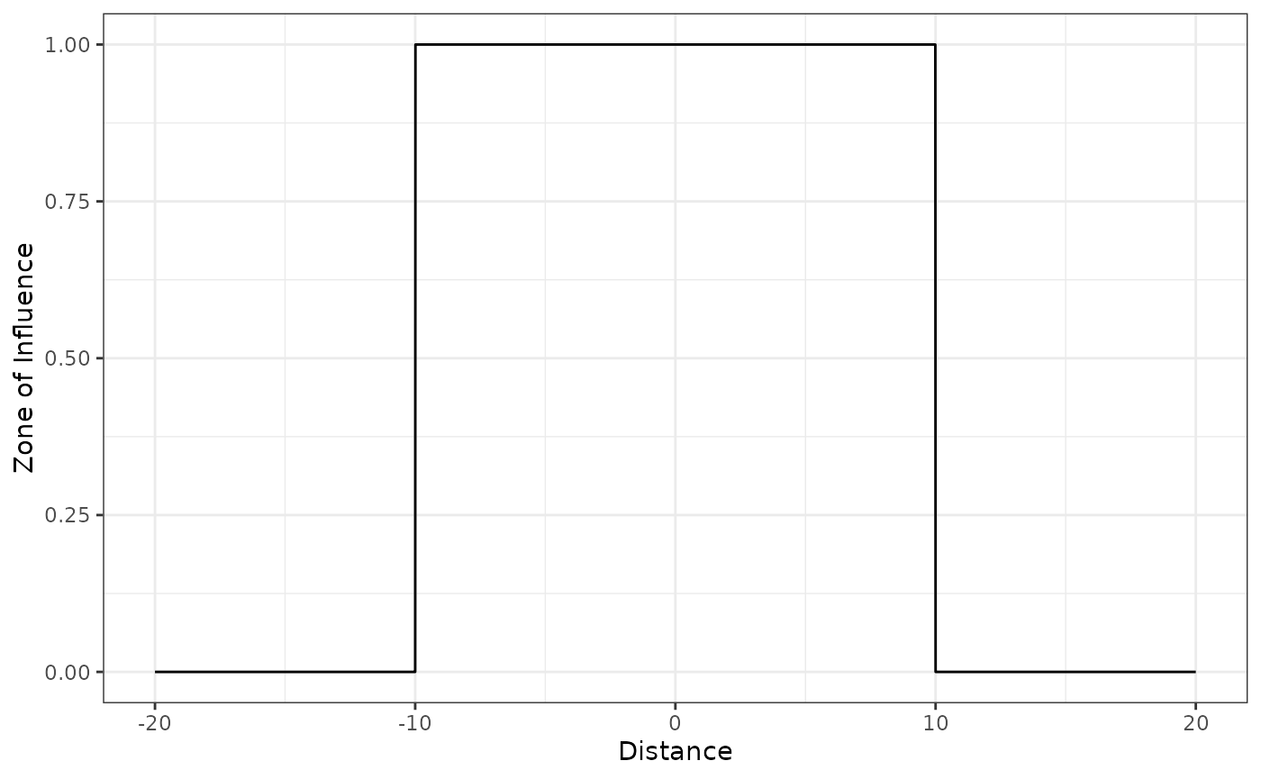
Linear decay function
The linear decay (also Bartlett or tent decay) function decreases
linearly with the distance
to infrastructure or source of disturbance and becomes zero at and
beyond the ZOI radius
.
It can be computed using the following functions:
linear_decay(), bartlett_decay(), and
tent_decay(). Here we show the use of the function:
# linear decay ZOI with radius = 10
linear_decay(5, radius = 10) # within the radius
#> [1] 0.5
linear_decay(10, radius = 10) # at or beyond the radius
#> [1] 0
We again visualize the function shape in 1 dimension space using the
function plot_zoi1d():
# threshold ZOI with radius = 10
plot_zoi1d(points = 0, radius = 10, fun = linear_decay, range_plot = c(-20, 20))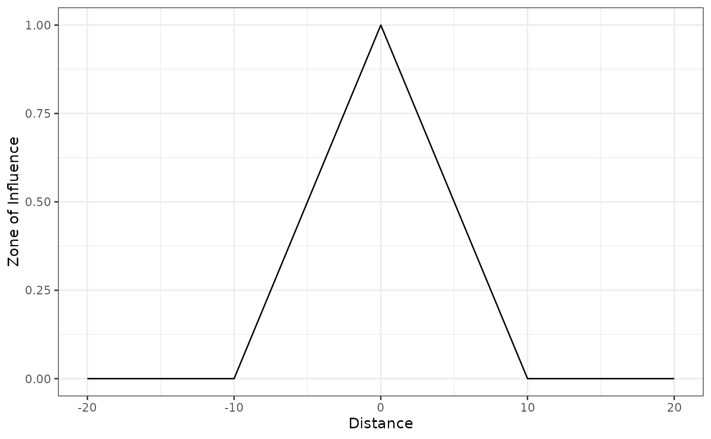
Functions that do not vanish with distance
Some functions decrease but do not vanish as the distance from
infrastructure increases. In these cases we define the ZOI radius
as the distance at which the ZOI decreases to
,
an arbitrary small ZOI value beyond which the influence of the
infrastructure is considered to be negligible. In these cases, the ZOI
definition needs an extra parameter and is defined as
.
Two functions of this type are implemented in oneimpact:
the exponential decay and the Gaussian decay functions.
Exponential decay function
The exponential decay function decays exponentially with the distance
to infrastructure, and the rate of decay is set so that
at the ZOI radius
().
The exponential decay might be calculated using the
exp_decay() function:
# exponential decay ZOI with radius = 10
exp_decay(5, radius = 10) # within the radius
#> [1] 0.2236068
exp_decay(10, radius = 10) # at the radius
#> [1] 0.05
exp_decay(15, radius = 10) # beyond the radius
#> [1] 0.01118034
As it is possible to see, an exponential decay ZOI with
radius = 10 does not imply the function is null beyond the
ZOI radius, but that it goes below the zoi_limit. By
default, zoi_limit = 0.05, but this value might be changed
by the user (e.g. to 0.01 or other small value). Changing
zoi_limit changes the interpretation of the ZOI radius
parameter, though:
# changing zoi_limit changes the interpretation of radius
exp_decay(5, radius = 10, zoi_limit = 0.01) # within the radius
#> [1] 0.1
exp_decay(10, radius = 10, zoi_limit = 0.01) # at the radius
#> [1] 0.01
exp_decay(15, radius = 10, zoi_limit = 0.01) # beyond the radius
#> [1] 0.001
We visualize the function shape in 1 dimension space:
# threshold ZOI with radius = 10
plot_zoi1d(points = 0, radius = 10, fun = exp_decay, range_plot = c(-20, 20)) +
  geom_hline(yintercept = 0.05, linetype = 2, color = "grey") +
  geom_vline(xintercept = c(-10, 10), linetype = 2, color = "grey")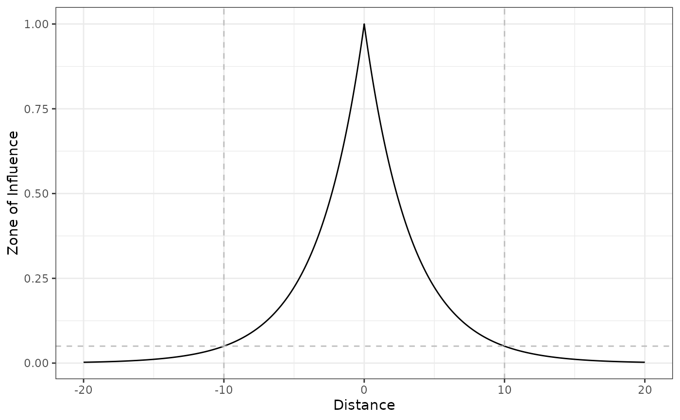
We add to the plot a horizontal dashed line at
zoi_limit = 0.05 and vertical dashed lines at
x = 10 and x = -10 (since
radius = 10), to show that the ZOI radius represents the
distance where the ZOI reaches zoi_limit.
Gaussian decay function
The Gaussian (or half-normal) decay function decays following a half
normal shape, and the rate of decay is set so that
at the ZOI radius
().
The Gaussian decay might be calculated using the
gaussian_decay() and half_norm_decay()
functions:
# Gaussian decay ZOI with radius = 10
gaussian_decay(5, radius = 10) # within the radius
#> [1] 0.4728708
gaussian_decay(10, radius = 10) # at or beyond the radius
#> [1] 0.05
gaussian_decay(15, radius = 10) # at or beyond the radius
#> [1] 0.001182177
We visualize the function shape in 1 dimension space:
# threshold ZOI with radius = 10
plot_zoi1d(points = 0, radius = 10, fun = gaussian_decay, range_plot = c(-20, 20)) +
  geom_hline(yintercept = 0.05, linetype = 2, color = "grey") +
  geom_vline(xintercept = c(-10, 10), linetype = 2, color = "grey")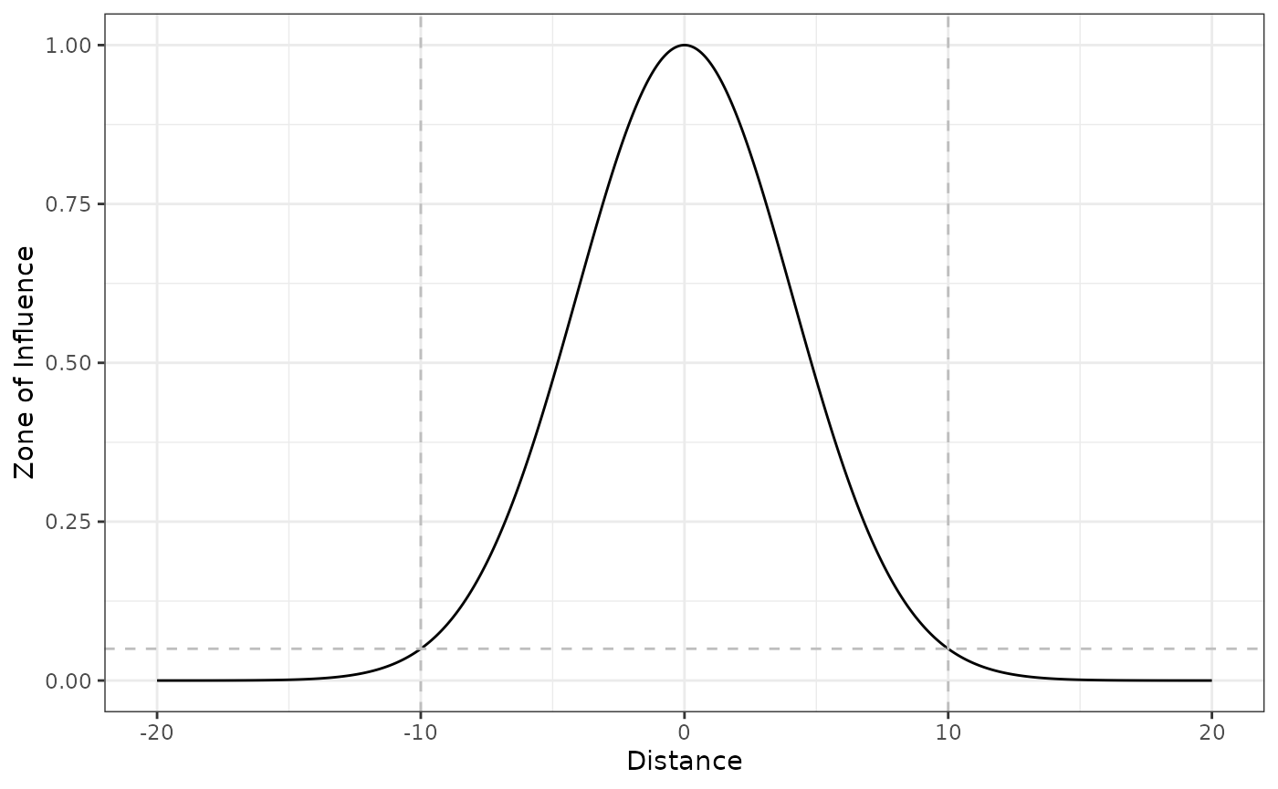
Notice that, even though the ZOI radius
is defined for all the functions, the change in their shape strongly
modifies the interpretation of how the ZOI changes with distance. These
functions set here might be used to calculate the ZOI of nearest feature
or to define weight matrices and calculate the cumulative ZOI of
multiple features. Alternatively, the generic function
dist_decay() can accomodate all these shapes by using the
argument type. For instance, to compute the ZOI of a
disturbance source following a linear decay shape with radius of 6, one
can use linear_decay(x = 0, radius = 6) or
dist_decay(x = 0, radius = 6, type = "linear").
ZOI metrics
Given a ZOI function was set with a specific shape and ZOI radius and there is more than one infrastructure feature or source of disturbance in space, two metrics might be calculated for the zone of influence: the ZOI of the nearest feature alone and the cumulative ZOI of multiple features.
To exemplify their difference, we illustrate them using a Gaussian
decay ZOI in 1 dimension space using the plot_zoi1d()
function. We set four sources of disturbance (e.g. houses) located at
x = 0, x = 2, x = 8, and
x = 12, and set the ZOI radius of each feature as
radius = 3. We start by plotting the ZOI of the nearest
feature alone by setting zoi_metric = "nearest":
disturbance_locations <- c(0, 2, 8, 12)
plot_zoi1d(points = disturbance_locations, radius = 3, fun = gaussian_decay,
           zoi_metric = "nearest", range_plot = c(-10, 20)) +
  labs(x = "Space") +
  ylim(0, 1.5) +
  geom_vline(xintercept = disturbance_locations, linetype = 2, color = "grey")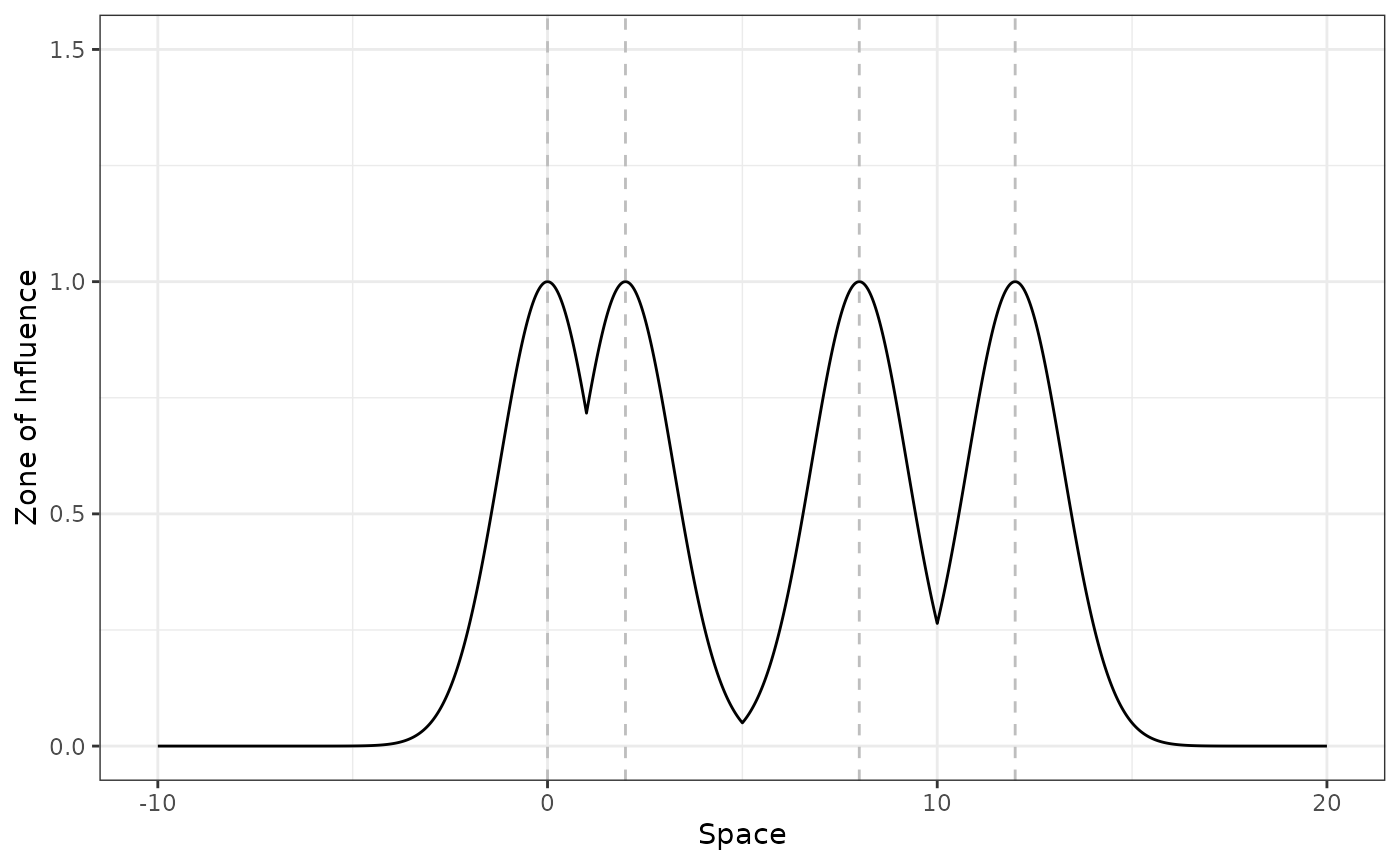
The location of the disturbance sources is shown by the vertical dashed lines. Notice that the the maximum value for the ZOI of the nearest feature is 1.
Now we do the same but considering that the ZOI of each feature
accumulates. We do it by setting zoi_metric = "cumulative"
in plot_zoi1d():
plot_zoi1d(points = disturbance_locations, radius = 3, fun = gaussian_decay,
           zoi_metric = "cumulative", range_plot = c(-10, 20)) +
  labs(x = "Space") +
  ylim(0, 1.5) +
  geom_vline(xintercept = disturbance_locations, linetype = 2, color = "grey")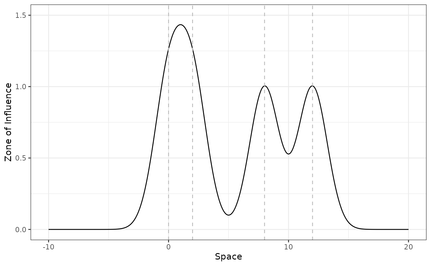
Notice that the the maximum value for the cumulative ZOI of multiple features might be higher than 1 where the ZOI of different features overlap.
Calculating the ZOI metrics for rasters
Define the input raster map
To calculate the ZOI metrics for 2 dimensional, raster objects, we
use the functions calc_zoi_nearest() and
calc_zoi_cumulative(). To give an example, we present a
data set with the location of private cabins in Norway, subset for a
small sample region in Southern Norway. The data is mapped as points in
vector format; more information about it might be found using the
command help(sample_area_cabins.gpkg). We read the vector
file using the package terra and plot it:
# file path
s <- system.file("vector/sample_area_cabins.gpkg", package = "oneimpact")
# read file
cabins_vect <- terra::vect(s)
# check
cabins_vect
#> class       : SpatVector
#> geometry    : points
#> dimensions  : 6875, 4  (geometries, attributes)
#> extent      : 146900.1, 194694.6, 6622822, 6658891  (xmin, xmax, ymin, ymax)
#> source      : sample_area_cabins.gpkg
#> coord. ref. : ETRS89 / UTM zone 33N (EPSG:25833)
#> names       :   cat buildtype  city value
#> type        : <int>     <chr> <int> <int>
#> values      :     1       161   604     1
#>                   2       161   604     1
#>                   3       161   604     1
#>               ...
# plot
plot(cabins_vect, cex = 0.5)
If the input map is already in raster format, it can be used directly
in the calc_zoi_*() functions. In our case, since it is in
vector format, it must be rasterized first. For many types of
anthropogenic infrastructure or disturbance which are represented by
lines or polygons (e.g. roads, power lines, areas of deforestation), it
is enough to create a binary raster as a dummy variable with value 1
where the disturbance is located and 0 (or NA) elsewhere
(see an example at this other oneimpact vignette).
For point representation of infrastructure and large enough pixels size,
though, it might be more interesting to count the number of features per
pixel, since there might be more than one feature within each pixel. To
create a raster with the number of cabins per pixel, we use the function
terra::rasterize() with parameter
fun = length. We load another raster with 100 m resolution
for the area to use it as a grid for the rasterization process.
# load grid
s2 <- system.file("raster/sample_area_cabins.tif", package = "oneimpact")
grid <- terra::rast(s2)
# rasterize
cabins_rast <- terra::rasterize(cabins_vect, grid, fun = length)
cabins_rast
#> class       : SpatRaster
#> size        : 361, 478, 1  (nrow, ncol, nlyr)
#> resolution  : 100, 100  (x, y)
#> extent      : 146900, 194700, 6622800, 6658900  (xmin, xmax, ymin, ymax)
#> coord. ref. : +proj=utm +zone=33 +ellps=GRS80 +units=m +no_defs
#> source(s)   : memory
#> varname     : sample_area_cabins
#> name        : V1
#> min value   :  1
#> max value   :  8
# plot
plot(cabins_rast)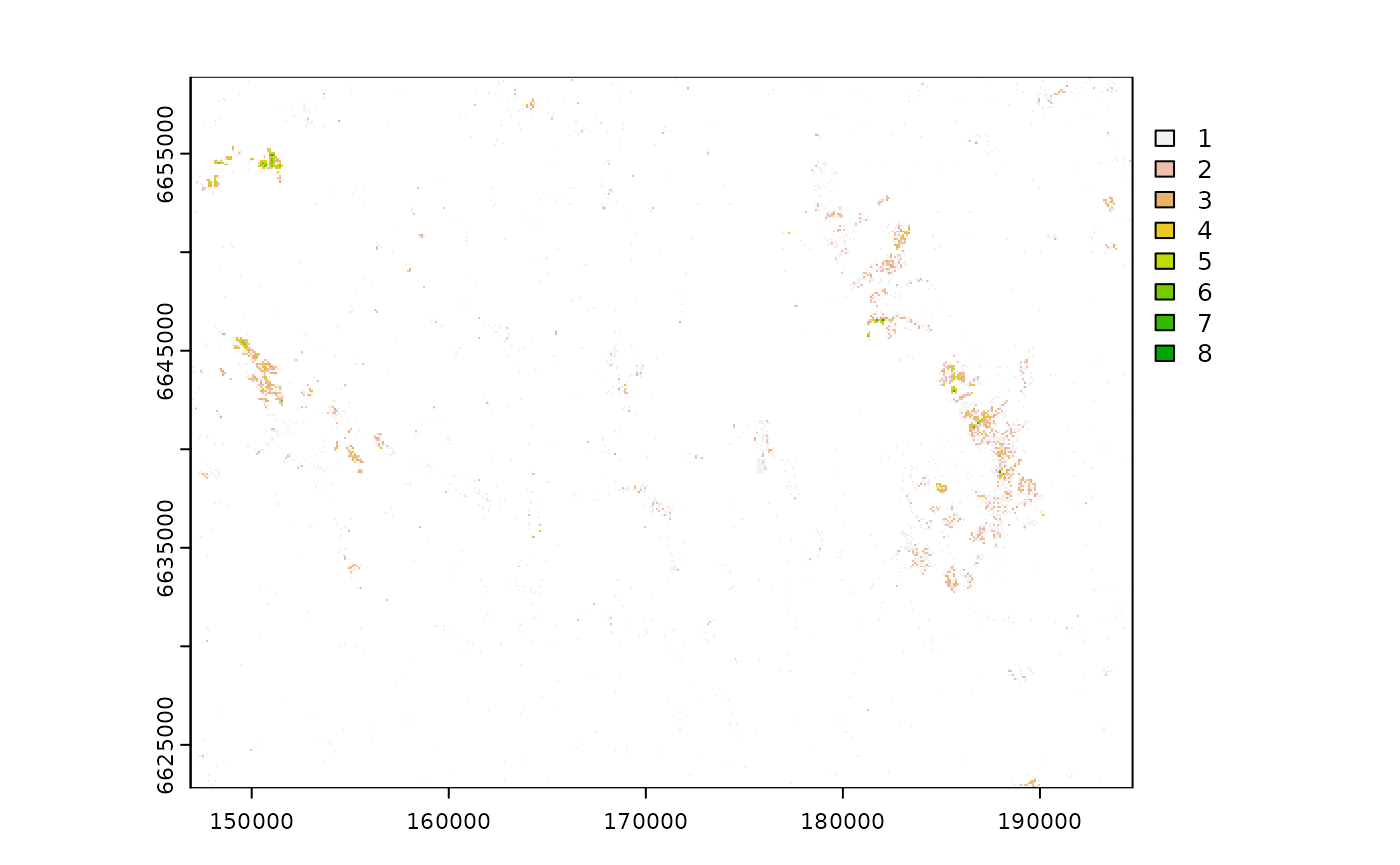
This map presents the number of cabins in each pixel and
NA where there are no cabins. As a similar procedure in
GRASS GIS, it is possible to use the ancillary oneimpact
function grass_v2rast_count() to count the number of
features of a vector in each pixel and get the output as a raster
object.
Compute the ZOI of the nearest feature only
This map might be used as it is as input for
calc_zoi_nearest(). For this function, is it important for
the background values of the input raster map (pixels with no cabins) to
be NA (no-data). We compute the ZOI of the nearest feature
using a Gaussian shaped ZOI with radius = 1000 m. By default, the
computation is done in R (parameter where = "R").
# calculate ZOI
cabins_nearest <- calc_zoi_nearest(cabins_rast, radius = 1000, type = "Gauss")
# plot
plot(cabins_nearest)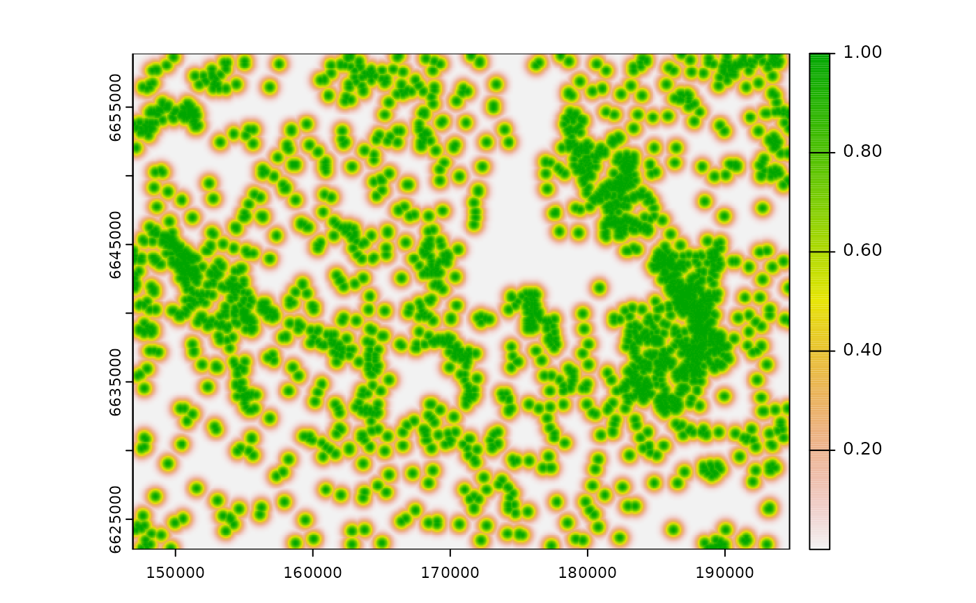
The shape of the ZOI might be changed through the parameter
type, using the functions presented above. This parameter
might be also set to type = "euclidean" for only the
computation of the Euclidean distance to the nearest feature or to
"log" or "sqrt" for the log- or
sqrt-transformed distance from the nearest feature.
Compute the cumulative ZOI of multiple features
Differently from calc_zoi_nearest(), the input raster
map for the calc_zoi_cumulative() should present zeros as
the background (pixels with no cabins). In R, background NA
values might be checked and reclassified to zero using the
zeroAsNA = TRUE parameter, but in GRASS GIS this is not
implemented. In this case, the easiest procedure is to prepare the input
raster map outside GRASS or make use of the module
[r.null](https://grass.osgeo.org/grass82/manuals/r.null.html)
for managing no-data values is rasters within GRASS. We calculate the
cumulative ZOI of multiple features using the same setup – a Gaussian
shaped ZOI with radius = 1000 m.
# calculate ZOI
cabins_cumul <- calc_zoi_cumulative(cabins_rast,
                                    radius = 1000,
                                    type = "gaussian_decay",
                                    zeroAsNA = TRUE)
# plot
plot(cabins_cumul)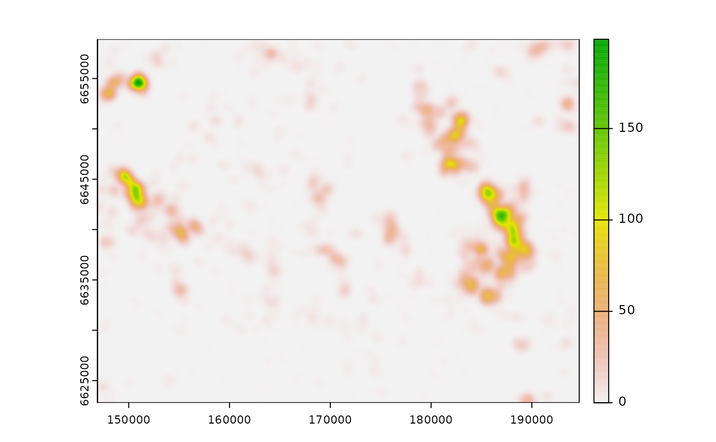
Notice that the output map differs considerably from the ZOI of the
nearest feature only. Here the shape of the ZOI might also be changed
through the parameter type, using the functions presented
above. Alternatively, a customized weight matrix might be defined by the
user and used as the radius parameter, in case which the
user must set type = "mfilter". Other functions to define
weight matrices might be set e.g. through terra::focalMat()
(Hijmans, 2022) or smoothie::kernel2dmeitsjer() (Gilleland,
2013) functions. Notice, however, that these functions are parameterized
differently, with no reference to the ZOI radius as the ones defined in
oneimpact.
For calc_zoi_cumulative(), the user might choose between
computing the cumulative ZOI metric when
output_type = "cumulative_zoi" (default), or the density of
features if output_type = "density". The cumulative ZOI is
the (distance weighted) number of features per unit of space, and might
assumes values much higher than one when there are features located
closer than the ZOI (see the illustrations above). The calculation of
the density of features, on the other hand, occurs after a normalization
of the weight matrix, so that its values sum 1. As a consequence, the
density of features generally presents values lower than or close to 1.
Both measures represent the same spatial variation, but the
interpretation of their values is different.
Using the ZOI approach to annotate and analyze data
In the cumulative impact assessment proposed in
oneimpact, the calculation of the ZOI
()
is done before statistical analysis. In this formulation,
defined based on different shapes and radii are considered as different
candidates of predictor variables in statistical models (see figure
below). Therefore, the evaluation of how the impact of multiple
infrastructure features accumulate and the identification of the ZOI
shape and radius are recasted as a model selection rather than a
parameterization problem.
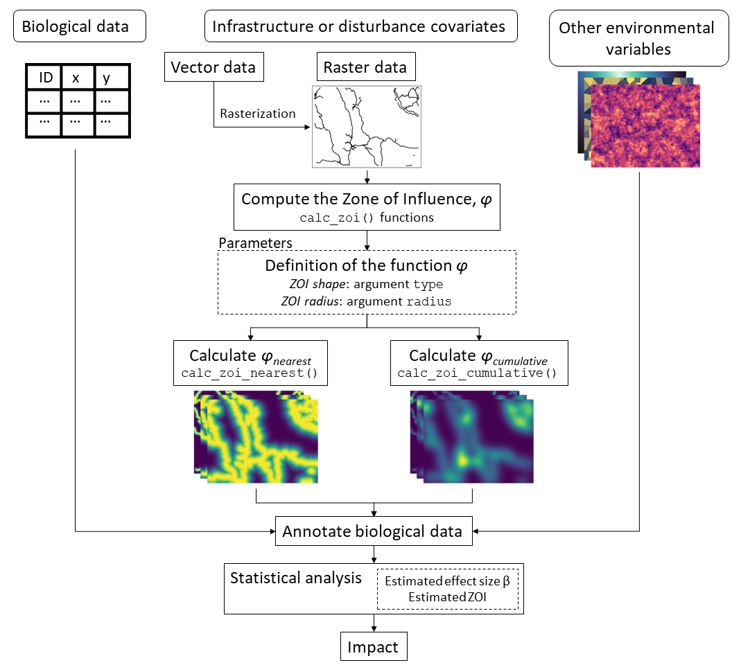
The figure above shows a workflow for calculating the ZOI metrics and
using them to annotate biological data for the estimation of cumulative
impacts. Infrastructure raster data are input to the
calc_zoi_*() functions, which allow the computation of the
ZOI of the nearest feaure and the cumulative ZOI based on arguments for
the ZOI shape and radius. The output influence rasters and other
environmental data are then annotated to biological data, and for each
infrastructure type each ZOI metric defined by a shape and radius is
considered as a different candidate for a predictor variable. The
annotated data is then analyzed through the statistical modeling
procedures selected by the user to estimate the effect size and the Zoi
radius for each infrastructure type and calculate the impact.
Here we simulate a data set of sampling points and a theoretical random biological response variable to show the process of calculation of ZOI variables and the annotation of the biological data.
First we create in the study area n = 40 random
locations representing sampling points for a given response variable
z (e.g. species richness or abundance). We sample the
locations using the set_points() function from the package
oneimpact and simulate the response variable z
as a Poisson distributed random variable with mean
.
The simulated sampled data is plotted below.
# seed
set.seed(111)
# get extent of the study area
extent <- terra::ext(cabins_rast)
# sample n = 40 random locations and simulate biological data
# get only coordinates with $pts at the end
bio_data <- set_points(40, method = "random", res = 100,
                       extent_x = extent[c(1,2)], extent_y = extent[c(3,4)])$pts |>
  sf::st_as_sf(coords = c(1,2), crs = crs(cabins_rast)) |> # change to sf object
  dplyr::mutate(id = 1:40, z = rpois(40, lambda = 10)) |> # add id and simulate response z
  terra::vect() # transform to vect to use with SpatRaster object
# plot
plot(cabins_vect, cex = 0.5)
plot(bio_data, col = "red", add = T)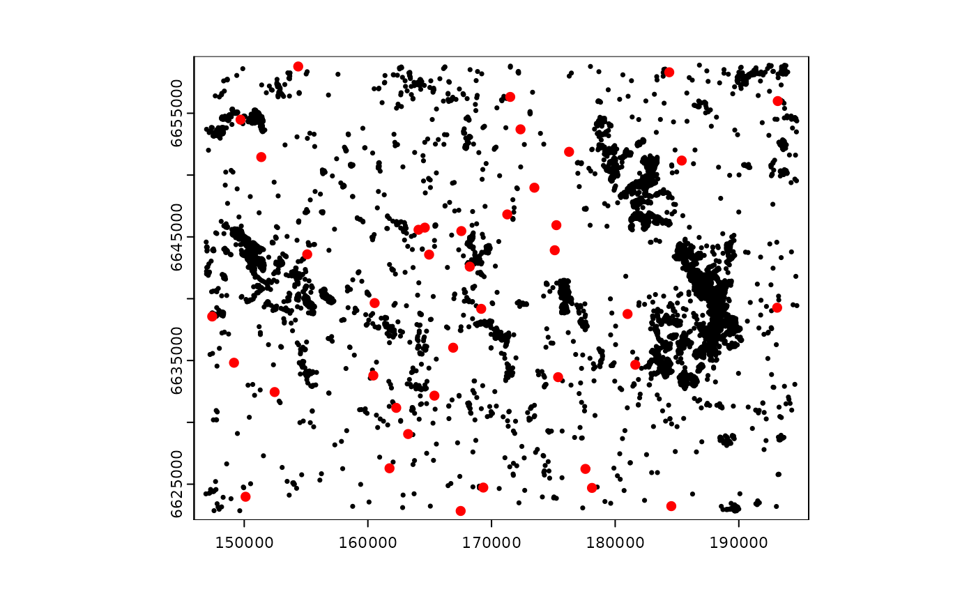
Now we use the same procedure presented above to calculate the ZOI of
the nearest feature and the cumulative ZOI for different radii. We use
an exponential decay ZOI and vary the ZOI radius from 500 m to 1500 m.
However, we use the calc_zoi() function which can compute
both ZOI metrics at once. To do so, we set the parameter
zeroAsNA to FALSE, since our input raster map
has NA as background values. We plot the ZOI layers
below.
# radii
radii <- c(500, 1000, 1500)
# exp decay ZOI - both nearest and cumulative
# use zeroAsNA = FALSE since the input has NULL as background
zoi_all <- oneimpact:::calc_zoi(cabins_rast,
                                radius = radii, type = "exp_decay",
                                zoi_metric = "all",
                                zeroAsNA = FALSE)
# plot
plot(zoi_all)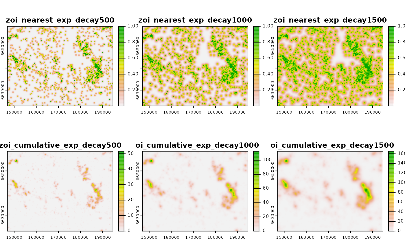
Finally, the ZOI variables can be used to annotate the biological data for statistical analysis.
# extract values
zoi_sampling_pts <- terra::extract(zoi_all, bio_data, )
# combine response variable with extracted data
bio_data_annotated <- dplyr::left_join(as.data.frame(bio_data, geom = "XY"),
                                       zoi_sampling_pts, by = c("id" = "ID"))
# show annotated data
head(bio_data_annotated)
#>   id  z        x       y zoi_nearest_exp_decay500 zoi_nearest_exp_decay1000
#> 1  1  6 175244.5 6645947             1.334868e-07              0.0003653584
#> 2  2  9 181625.8 6634659             4.711992e-02              0.2170712325
#> 3  3  8 164606.2 6645748             8.455576e-02              0.2907847396
#> 4  4 11 171513.4 6656320             1.152959e-01              0.3395525377
#> 5  5 10 164952.3 6643566             1.445658e-02              0.1202355317
#> 6  6 13 166896.5 6636037             1.088078e-04              0.0104310997
#>   zoi_nearest_exp_decay1500 _zoi_cumulative_exp_decay500
#> 1               0.005110688                   0.00000000
#> 2               0.361189277                   0.08906389
#> 3               0.438915658                   0.12350292
#> 4               0.486711178                   0.18623277
#> 5               0.243606320                   0.03573248
#> 6               0.047740474                   0.00000000
#>   _zoi_cumulative_exp_decay1000 _zoi_cumulative_exp_decay1500
#> 1                    0.00000000                    0.02269499
#> 2                    1.16104432                    4.87939875
#> 3                    0.88921937                    2.34383617
#> 4                    0.88243528                    1.75187108
#> 5                    0.38080083                    1.07029764
#> 6                    0.04619249                    0.45860291
From this point, biological data can also be annotated with the ZOI
of other disturbance variables and with other environmental covariates
and used as input for the estimation of the effect sizes
and evaluation of the cumulative effects for different types of
infrastructure through statistical models. Statistical analyses can make
use of model selection (Burnham & Anderson, 2002; Jackson &
Fahrig, 2015; Huais, 2018), penalized regression (Lee et al., 2020), or
machine learning approaches, for example (James et al., 2021). Such
statistical modeling procedures are beyond the scope of
oneimpact.
References
Bivand, R. (2022). rgrass7: Interface Between GRASS Geographical Information System and R. R package version 0.2-10. https://CRAN.R-project.org/package=rgrass7
Burnham, K. P., & Anderson, D. R. (2002). Model selection and multimodel inference: A practical information-theoretic approach (2nd ed). Springer.
Gilleland, E. (2013). Two-dimensional kernel smoothing: Using the R package smoothie. NCAR Technical Note, TN-502+STR, 17pp., doi:10.5065/D61834G2.
GRASS Development Team (2017) Geographic Resources Analysis Support System (GRASS GIS) Software, Version 7.8. Open Source Geospatial Foundation.
Hijmans, R. J. (2022). terra: Spatial Data Analysis. R package version 1.5-21. https://CRAN.R-project.org/package=terra
Huais, P. Y. (2018). multifit: An R function for multi-scale analysis in landscape ecology. Landscape Ecology, 33(7), 1023–1028. https://doi.org/10.1007/s10980-018-0657-5
Jackson, H. B., & Fahrig, L. (2015). Are ecologists conducting research at the optimal scale? Global Ecology and Biogeography, 24(1), 52–63. https://doi.org/10.1111/geb.12233
James, G., Witten, D., Hastie, T., & Tibshirani, R. (2021). An introduction to statistical learning: With applications in R (Second edition). Springer.
Lee, Y., Alam, M., Sandström, P., & Skarin, A. (2020). Estimating zones of influence using threshold regression. Working Papers in Transport, Tourism, Information Technology and Microdata Analysis, 2020:01, 1–16.
Miguet, P., Jackson, H. B., Jackson, N. D., Martin, A. E., & Fahrig, L. (2016). What determines the spatial extent of landscape effects on species? Landscape Ecology, 31(6), 1177–1194. https://doi.org/10.1007/s10980-015-0314-1
Miguet, P., Fahrig, L., & Lavigne, C. (2017). How to quantify a distance‐dependent landscape effect on a biological response. Methods in Ecology and Evolution, 8(12), 1717–1724. https://doi.org/10.1111/2041-210X.12830
Niebuhr, B. B., van Moorter, B., Stien, A., Tveraa, T., Strand, O., Langeland, K., Alam, M., Skarin, A., & Panzacchi, M. Estimating the cumulative impact and zone of influence of anthropogenic infrastructure on biodiversity. Methods in Ecology and Evolution, 14, 2362–2375. https://doi.org/10.1111/2041-210X.14133
R Core Team (2021). R: A language and environment for statistical computing. R Foundation for Statistical Computing, Vienna, Austria. https://www.R-project.org/.