Calculate the cumulative zone of influence of multiple features
Source:R/calc_zoi_cumulative.R
calc_zoi_cumulative.RdThis function takes in a raster with locations or counts of
infrastructure
and calculates a raster (or set of rasters, in case there is more the one
value for radius) representing the cumulative zone of influence (ZOI)
or density of features in space. The process is done through a spatial
filter/moving window/neighborhood analysis. The zones of influence
(or weight matrices) are defined by functions that decay with the distance
from each infrastructure feature and their rate of decay is controlled by the
ZOI radius (radius), which defines how far the influence of an infrastructure
feature goes. By using moving window analyses, the cumulative ZOI account for
the sum of the influence of multiple features across space, weighted by
the distance to these features according the the ZOI shape.
For more details on the ZOI functions, see zoi_functions().
The procedure might be computed in both R and GRASS GIS. In R, the
neighborhood analysis is done with the terra::focal() function. In GRASS,
different modules might be used for the computation: r.resamp.filter,
r.mfilter, or r.neighbors. See details for their differences. In GRASS, it
requires an active connection between the R session and a GRASS GIS
location and mapset (through the package rgrass), and that the input
maps are already loaded within this GRASS GIS mapset.
If the calculations are done in R, the input is a (set of) raster map(s)
and the function returns another (set of) raster map(s). If the calculations
are done within GRASS GIS, the input is the name of a raster map already
loaded in a GRASS GIS location and mapset, and the function returns
only the name of the output map. This map is stored in the the GRASS GIS
location/mapset, and might be retrieved to R through the
rgrass::read_RAST() function or exported outside GRASS using the
r.out.gdal module, for instance.
Usage
calc_zoi_cumulative(
  x,
  radius = 100,
  type = c("circle", "Gauss", "rectangle", "exp_decay", "bartlett", "threshold",
    "mfilter")[1],
  where = c("R", "GRASS")[1],
  output_type = c("cumulative_zoi", "density")[1],
  zoi_limit = 0.05,
  min_intensity = 0.01,
  max_dist = 50000,
  zeroAsNA = FALSE,
  extent_x_cut = NULL,
  extent_y_cut = NULL,
  na.policy = "omit",
  na.rm = TRUE,
  g_module = c("r.mfilter", "r.resamp.filter", "r.neighbors")[1],
  g_parallel = TRUE,
  g_output_map_name = NULL,
  g_input_as_region = FALSE,
  g_remove_intermediate = TRUE,
  g_overwrite = FALSE,
  verbose = FALSE,
  ...
)
Arguments
- x
[RasterLayer,SpatRaster,character]
Raster representing locations of features, preferentially with positive values where the features are located (or counts of features within a pixel) and 0 elsewhere. Alternatively,xmight be a binary (dummy) spatial variable representing the presence of linear or area features, with zero as background.xcan be aRasterLayerfrom raster package or a SpatRaster from terra package. Ifwhere = "GRASS",xmust be a string corresponding to the name of the input map within a GRASS GIS location and mapset. Continuous or discrete raster maps with multiple categories can be binarized to be used as input forcalc_zoi_cumulative()throughgrass_binarize()in GRASS GIS, or through common raster algebra in both R and GRASS.Notice that, different from
calc_zoi_nearest(), the input mapsxmust have zero as background values, instead of NA. In R it is possible to account for NA background values by settingzeroAsNA = TRUEfor the computation of the cumulative ZOI. In GRASS, maps without NA as background might be changed into maps with 0 as background to be used incalc_zoi_cumulative()through raster algebra and e.g. through the use of the moduler.null.- radius
[numeric(1)=100]
Radius or scale of the moving window for neighborhood analysis, used to calculate the cumulative zoi and density. The radius represent the distance at which the ZOI vanishes or goes below a given minimum limit valuezoi_limit. It can be a single value or a vector of values, in which case several cumulative ZOI or density maps (one for each radius) are created. Fortype = "circle", theradiuscorresponds to the radius of the circle filter. Fortype = "Gauss"andtype = "exp_decay",radiuscorresponds to the distance where the Gaussian or exponential decay function decrease or a smallzoi_limitvalue. Iftype = "bartlett",radiusis the distance at which the filter reaches zero, after a linear decay from the central pixel. Iftype = "rectangle",radiuscorresponds to half the size of the side of a square filter. Iftype = "mfilter", radius is not a numeric value but a matrix itself, defined by the user. See description in the details andzoi_functions()for more details on the zone of influence function shapes and parameters.- type
[character(1)="circle"]{"circle", "Gauss", "rectangle", "exp_decay", "bartlett", "threshold", "step", "mfilter"}
Type of filter (shape of the zone of influence) used to calculate the cumulative ZOI or density. See details.- where
[character(1)="R"]{"R", "GRASS"}
Where should the computation be done? Default is"R". Ifwhere = "GRASS", the R session must be linked to an open GRASS GIS session in a specific location and mapset.- output_type
[character(1)="cumulative_zoi"]{"cumulative_zoi", "density"}
Ifoutput_type = "cumulative_zoi"(default), the ZOI weight matrix not not normalized, i.e. the maximum value of the weight matrix at the central pixel value is always 1. This means the values of the input map are summed (considering a decay with distance within the neighborhood) and the output map presents values higher than 1. Ifoutput_type = "density", the weight matrix is normalized before the filtering process, leading to values in the outmap map generally lower than 1.- zoi_limit
[numeric(1)=0.05]
For non-vanishing functions (e.g.exp_decay,gaussian_decay), this value is used to set the relationship between the ZOI radius and the decay functions:radiusis defined as the minimum distance at which the ZOI assumes values belowzoi_limit. The default is 0.05. This parameter is used only ifradiusis notNULL.- min_intensity
[numeric(1)=0.01]
Minimum intensity of the exponential and Gaussian decay functions to define the radius of the window that define the filter. Seefilter_create()for details.- max_dist
[numeric(1)=50000]
Maximum size (in meters) to define the radius of the window that defines the filter. Only applicable for exponential and Gaussian decay functions. Seefilter_create()for details.- zeroAsNA
[logical(1)=FALSE]
IfTRUEtreats cells that areNAas if they were zero.- extent_x_cut, entent_y_cut
[numeric vector(2)=c(0,1)]
Vector representing the minimum and maximum extent in x and y for the final output, in the format c(min,max). It is intended to keep only a region of interest but consider the surroundings when calculating the cumulative ZOI or density. This might be especially useful for example in the use of ther.mfilteralgorithm in GRASS, in which the edges of the region are excluded from the computation. The default is to keep the same extent of the input raster.- na.policy
[character(1)="omit"]
Can be used to determine the cells ofxfor which focal values should be computed. Must be one of "all" (compute for all cells), "only" (only for cells that are NA) or "omit" (skip cells that are NA). Note that the value of this argument does not affect which cells around each focal cell are included in the computations (use na.rm=TRUE to ignore cells that are NA for that). Seeterra::focal()for details. Only used whenwhere = "R".- na.rm
[logical(1)=FALSE]
Should missing values be removed for filtering calculations? Option for the neighborhood analysis performed through theterra::focal()function. Only used whenwhere = "R".- g_module
[character(1)="r.mfilter"]{"r.mfilter", "r.resamp.filter", "r.neighbors"}
Ifwhere = "GRASS", which algorithm should be used to compute the cumulative ZOI? See details for their description.- g_parallel
[logical(1)=TRUE]
If ther.mfiltertool is used for computing the cumulative ZOI in GRASS GIS,g_paralleltells if parallelization should be used. Default isTRUE. The option is ignored for other GRASS tools (parameterg_module) and for computation in R (where = "R").- g_output_map_name
[character(1)=NULL]
Name of the output map. Only used whenwhere = "GRASS". IfNULL(default), a standard name is created based on the name of the input mapx, the ZOI shapetype, and the ZOI radiusradius.- g_input_as_region
[logical(1)=TRUE]
Should the input mapxbe used to redefine the working GRASS region before cumulative ZOI calculation? IfTRUE,xis used to define the region withg.region. IfFALSE, the region previously defined in the GRASS GIS session is used for computation.- g_remove_intermediate
[logical(1)=TRUE]
Should the intermediate maps created for computing the output map be excluded in the end of the process? Only used whenwhere = "GRASS".- g_overwrite
[logical(1)=FALSE]
If the a map already exists with the nameg_output_map_namein the working GRASS GIS location and mapset, should it be overwritten? Only used whenwhere = "GRASS".- verbose
[logical(1)=FALSE]
Should messages of the computation steps be printed in the prompt along the computation?- ...
Other arguments to be used within
filter_create()orterra::focal().
Value
If the calculations are performed in R (where = "R"),
a RasterLayer or SpatRaster (according to the input x map)
with the cumulative zone of influence or density of features. While the
cumulative ZOI uses a ZOI/weight matrix rescaled to 1 at the central pixel
(creating values in the output map which might go well beyond 1), the
density of features uses a normalized ZOI/weight matrix (with all values
summing 1), what created values smaller than one in the output map.
if multiple radius values are given, a RasterBrick or multi-layer
SpatRaster, with the cumulative ZOI or density maps for each ZOI radius.
If the computation is done in GRASS GIS, the output is the name of
the output raster map(s) within the GRASS GIS location and mapset of the
current session. The user can retrieve these maps to R using
rgrass::read_RAST() or export them outside GRASS using the
r.out.gdal module, for instance.
Details
The input raster is supposed to represent the location of point, line, or polygon infrastructure (e.g. houses, roads, mining areas), but any landscape variable whose representation might be one of those would fit here (e.g. areas of forest or any other habitat type or land cover). We recommend that the input raster has a metric projection, so that distances and zones of influence are based on distance to infrastructure measured in meters.
Zone of Influence functions and weight matrices
The neighborhood analysis to define the cumulative ZOI can be computed with different functions/filters. The options currently implemented are:
circular/threshold matrix: the circular filter (
type = "circle"ortype = "threshold"ortype = "step") is a matrix with constant weights in which the parameterradiuscorresponds to the radius of the circle centered on the central pixel. It is similar to a circular buffer matrix.Gaussian matrix: the Gaussian filter (
type = "Gauss"ortype = "gauss"ortype = "gaussian_decay") is a matrix with weights following a Gaussian or Normal decay. The Gaussian curve is 1 at the central cell and is parameterized on theradiusand thezoi_limit, which controls how fast the curve decreases with distance. Seezoi_functions()for details.Exponential decay matrix: the exponential decay filter (
type = "exp_decay") is a matrix with weights following an exponential decay curve, with value 1 in the central cell and parameterized on theradiusand thezoi_limit. Seezoi_functions()for details.Rectangular matrix: the rectangular filter (
type = "rectangle"ortype = "box") is a weight matrix whose shape is a square of dimensions \(n\) x \(n\), with \(n = 2 * radius\).Bartlett or linear decay matrix: the Bartlett, linear, or tent decay filter (
type = "bartlett"ortype = "linear_decay"ortype = "tent_decay") is a weight matrix whose value is 1 in the central cell and whose weights decrease linearly up to zero at a distance equalsradius. Seezoi_functions()for details.user-customized filter: if
type = "mfilter",radiusis not numeric but should be a user-defined matrix of weights. Examples are ones created throughfilter_create(),terra::focalMat(),smoothie::kernel2dmeitsjer(), or matrices created by hand.
Weight matrices might differ from the expected decay function depending on the intended resolution - the finer the resolution, the more detailed and correspondent to the original functions the matrix will be.
Algorithms in GRASS GIS
In GRASS GIS, different modules might be used for the computation,
r.resamp.filter, r.mfilter, or r.neighbors. The module to be used is
controlled by the parameter g_module. These algorithms provide different
capabilities and flexibility.
r.resamp.filterseems to be the fastest one in most cases, but has less flexibility in the choice of the zone of influence function. The algorithm calculates the weighted density of features, which might be rescaled to the cumulative ZOI if the appropriate scaling factor (calculated from the weight matrix) is provided. Currently only the filterstype = "bartlett"andtype = "box"are implemented. More information about the algorithm here.r.mfilteris slower thanr.resamp.filterbut much faster thanr.neighbors, and allows a flexible choice of the shape of the zone of influence (the wight matrix shape).r.mfilteris then the most indicated in terms of a balance between flexibility in the choice of the ZOI shape and computation efficiency. The only inconvenient ofr.mfilteris that it creates an edge effect with no information in the outer cells of a raster (the number of cells correspond toradiusor half the size of the weight matrix), so if it is used the users should add a buffer area
= radius around the input raster map, to avoid such edge effects.See https://github.com/OSGeo/grass/issues/2184 for more details.
r.neighborsis considerably slower than the other algorithms (from 10 to 100 times), but allows a flexible choice of the ZOI shape. Contrary tor.resamp.filterandr.mfilter, which can only perform a sum of pixel values weighted by the input filter or ZOI,r.neighborsmight calculate many other statistical summaries within the window of analysis, such as mean, median, standard deviation etc.
See also
See zoi_functions() for some ZOI function shapes and
filter_create() for options to create weight matrices.
See also smoothie::kernel2dmeitsjer(), terra::focalMat(), and
raster::focalWeight() for other functions to create filters or weight matrices.
See
r.mfilter,
r.resamp.filter, and
r.neighbors for
GRASS GIS implementations of neighborhood analysis.
See calc_zoi_nearest() for the computation of the zone of influence
of the nearest feature only.
Examples
# Running calc_zoi_cumulative through R
library(terra)
# Load raster data
f <- system.file("raster/sample_area_cabins_count.tif", package = "oneimpact")
cabins <- terra::rast(f)
# calculate cumulative zone of influence for multiple influence radii,
# using a Gaussian filter
zoi_values <- c(250, 500, 1000, 2500, 5000)
cumzoi_gauss <- calc_zoi_cumulative(cabins, type = "Gauss", radius = zoi_values)
plot(cumzoi_gauss)
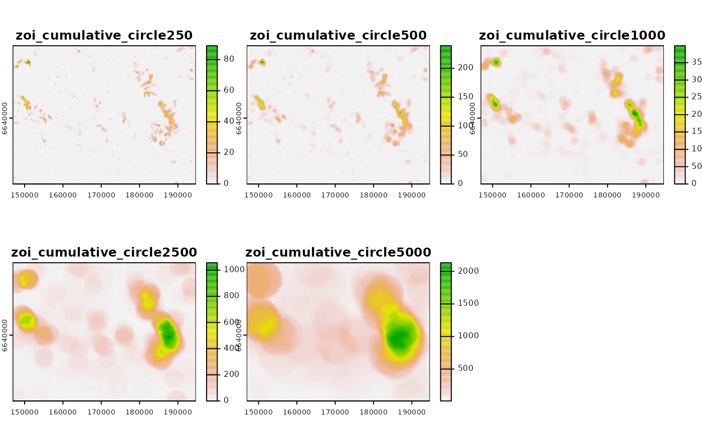
 # calculate cumulative zone of influence for multiple influence radii,
# using a circle neighborhood
cumzoi_circle <- calc_zoi_cumulative(cabins, type = "circle", radius = zoi_values)
plot(cumzoi_circle)
# calculate cumulative zone of influence for multiple influence radii,
# using a circle neighborhood
cumzoi_circle <- calc_zoi_cumulative(cabins, type = "circle", radius = zoi_values)
plot(cumzoi_circle)
 # calculate cumulative zone of influence for multiple influence radii,
# using an exponential decay neighborhood
cumzoi_exp <- calc_zoi_cumulative(cabins, type = "exp_decay", radius = zoi_values)
plot(cumzoi_exp)
# calculate cumulative zone of influence for multiple influence radii,
# using an exponential decay neighborhood
cumzoi_exp <- calc_zoi_cumulative(cabins, type = "exp_decay", radius = zoi_values)
plot(cumzoi_exp)
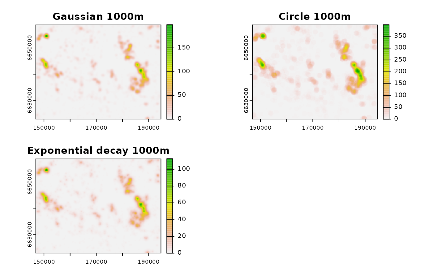
 # comparing
plot(c(cumzoi_gauss[[3]], cumzoi_circle[[3]], cumzoi_exp[[3]]),
main = c("Gaussian 1000m",
"Circle 1000m",
"Exponential decay 1000m"))
# comparing
plot(c(cumzoi_gauss[[3]], cumzoi_circle[[3]], cumzoi_exp[[3]]),
main = c("Gaussian 1000m",
"Circle 1000m",
"Exponential decay 1000m"))
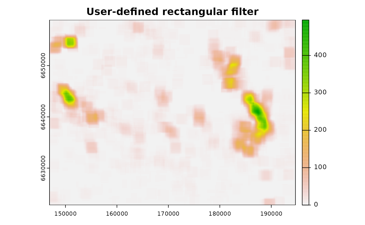
 # calculate cumulative influence for a single zone of influence
# using a user-defined filter
my_filter <- filter_create(cabins, radius = 1000, type = "rectangle")
cumzoi_user <- calc_zoi_cumulative(cabins, type = "mfilter", radius = my_filter)
plot(cumzoi_user, main = "User-defined rectangular filter")
# calculate cumulative influence for a single zone of influence
# using a user-defined filter
my_filter <- filter_create(cabins, radius = 1000, type = "rectangle")
cumzoi_user <- calc_zoi_cumulative(cabins, type = "mfilter", radius = my_filter)
plot(cumzoi_user, main = "User-defined rectangular filter")
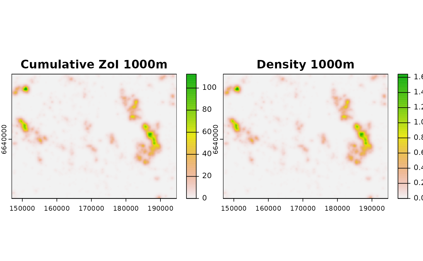
 # calculate density with 1000m radius using an exp_decay neighborhood
density_exp <- calc_zoi_cumulative(cabins, type = "exp_decay", radius = 1000,
output_type = "density")
# compare
# note the difference in the color scales
plot(c(cumzoi_exp[[3]], density_exp),
main = c("Cumulative ZoI 1000m", "Density 1000m"))
# calculate density with 1000m radius using an exp_decay neighborhood
density_exp <- calc_zoi_cumulative(cabins, type = "exp_decay", radius = 1000,
output_type = "density")
# compare
# note the difference in the color scales
plot(c(cumzoi_exp[[3]], density_exp),
main = c("Cumulative ZoI 1000m", "Density 1000m"))
 #--------------------
# Running calc_zoi_cumulative through GRASS GIS
library(rgrass)
#> GRASS GIS interface loaded with GRASS version: (GRASS not running)
library(terra)
# Load raster data
f <- system.file("raster/sample_area_cabins.tif", package = "oneimpact")
cabins <- terra::rast(f)
# connect to grass gis and create grass location
# For linux or within OSGeo4W shell
grassdir <- system("grass --config path", intern = TRUE)
# grassdir <- system("grass78 --config path", intern = TRUE) # for GRASS 7.8
# If you used the standalone installer in Windows
# grassdir <- "C:\Programs\GRASS GIS 7.8" # Correct if the path GRASS version or path is different
gisDB <- "." # create location and mapset in the working directory
loc <- "ETRS_33N/" # name of the location
ms <- "PERMANENT" # name of the mapset
rgrass::initGRASS(gisBase = grassdir,
SG = cabins, # use map to define location projection
home = tempdir(),
override = TRUE,
gisDbase = gisDB,
location = loc,
mapset = ms)
#> gisdbase .
#> location ETRS_33N/
#> mapset PERMANENT
#> rows 361
#> columns 478
#> north 6658900
#> south 6622800
#> west 146900
#> east 194700
#> nsres 100
#> ewres 100
#> projection:
#> PROJCRS["unknown",
#> BASEGEOGCRS["grs80",
#> DATUM["European Terrestrial Reference System 1989",
#> ELLIPSOID["Geodetic_Reference_System_1980",6378137,298.257222101,
#> LENGTHUNIT["metre",1]],
#> ID["EPSG",6258]],
#> PRIMEM["Greenwich",0,
#> ANGLEUNIT["degree",0.0174532925199433,
#> ID["EPSG",9122]]]],
#> CONVERSION["Transverse Mercator",
#> METHOD["Transverse Mercator",
#> ID["EPSG",9807]],
#> PARAMETER["Latitude of natural origin",0,
#> ANGLEUNIT["degree",0.0174532925199433],
#> ID["EPSG",8801]],
#> PARAMETER["Longitude of natural origin",15,
#> ANGLEUNIT["degree",0.0174532925199433],
#> ID["EPSG",8802]],
#> PARAMETER["Scale factor at natural origin",0.9996,
#> SCALEUNIT["unity",1],
#> ID["EPSG",8805]],
#> PARAMETER["False easting",500000,
#> LENGTHUNIT["metre",1],
#> ID["EPSG",8806]],
#> PARAMETER["False northing",0,
#> LENGTHUNIT["metre",1],
#> ID["EPSG",8807]]],
#> CS[Cartesian,2],
#> AXIS["easting",east,
#> ORDER[1],
#> LENGTHUNIT["metre",1,
#> ID["EPSG",9001]]],
#> AXIS["northing",north,
#> ORDER[2],
#> LENGTHUNIT["metre",1,
#> ID["EPSG",9001]]]]
# define map name within GRASS GIS
cabins_g <- "cabins_example"
# add file to GRASS GIS mapset
rgrass::write_RAST(cabins, cabins_g, flags = c("o", "overwrite"))
#> Over-riding projection check
#> Importing raster map <cabins_example>...
#> 0% 3% 6% 9% 12% 15% 18% 21% 24% 27% 30% 33% 36% 39% 42% 45% 48% 51% 54% 57% 60% 63% 66% 69% 72% 75% 78% 81% 84% 87% 90% 93% 96% 99% 100%
#> SpatRaster read into GRASS using r.in.gdal from file
# check
terra::plot(cabins, col = "black",
main = "Map of tourist cabins")
#--------------------
# Running calc_zoi_cumulative through GRASS GIS
library(rgrass)
#> GRASS GIS interface loaded with GRASS version: (GRASS not running)
library(terra)
# Load raster data
f <- system.file("raster/sample_area_cabins.tif", package = "oneimpact")
cabins <- terra::rast(f)
# connect to grass gis and create grass location
# For linux or within OSGeo4W shell
grassdir <- system("grass --config path", intern = TRUE)
# grassdir <- system("grass78 --config path", intern = TRUE) # for GRASS 7.8
# If you used the standalone installer in Windows
# grassdir <- "C:\Programs\GRASS GIS 7.8" # Correct if the path GRASS version or path is different
gisDB <- "." # create location and mapset in the working directory
loc <- "ETRS_33N/" # name of the location
ms <- "PERMANENT" # name of the mapset
rgrass::initGRASS(gisBase = grassdir,
SG = cabins, # use map to define location projection
home = tempdir(),
override = TRUE,
gisDbase = gisDB,
location = loc,
mapset = ms)
#> gisdbase .
#> location ETRS_33N/
#> mapset PERMANENT
#> rows 361
#> columns 478
#> north 6658900
#> south 6622800
#> west 146900
#> east 194700
#> nsres 100
#> ewres 100
#> projection:
#> PROJCRS["unknown",
#> BASEGEOGCRS["grs80",
#> DATUM["European Terrestrial Reference System 1989",
#> ELLIPSOID["Geodetic_Reference_System_1980",6378137,298.257222101,
#> LENGTHUNIT["metre",1]],
#> ID["EPSG",6258]],
#> PRIMEM["Greenwich",0,
#> ANGLEUNIT["degree",0.0174532925199433,
#> ID["EPSG",9122]]]],
#> CONVERSION["Transverse Mercator",
#> METHOD["Transverse Mercator",
#> ID["EPSG",9807]],
#> PARAMETER["Latitude of natural origin",0,
#> ANGLEUNIT["degree",0.0174532925199433],
#> ID["EPSG",8801]],
#> PARAMETER["Longitude of natural origin",15,
#> ANGLEUNIT["degree",0.0174532925199433],
#> ID["EPSG",8802]],
#> PARAMETER["Scale factor at natural origin",0.9996,
#> SCALEUNIT["unity",1],
#> ID["EPSG",8805]],
#> PARAMETER["False easting",500000,
#> LENGTHUNIT["metre",1],
#> ID["EPSG",8806]],
#> PARAMETER["False northing",0,
#> LENGTHUNIT["metre",1],
#> ID["EPSG",8807]]],
#> CS[Cartesian,2],
#> AXIS["easting",east,
#> ORDER[1],
#> LENGTHUNIT["metre",1,
#> ID["EPSG",9001]]],
#> AXIS["northing",north,
#> ORDER[2],
#> LENGTHUNIT["metre",1,
#> ID["EPSG",9001]]]]
# define map name within GRASS GIS
cabins_g <- "cabins_example"
# add file to GRASS GIS mapset
rgrass::write_RAST(cabins, cabins_g, flags = c("o", "overwrite"))
#> Over-riding projection check
#> Importing raster map <cabins_example>...
#> 0% 3% 6% 9% 12% 15% 18% 21% 24% 27% 30% 33% 36% 39% 42% 45% 48% 51% 54% 57% 60% 63% 66% 69% 72% 75% 78% 81% 84% 87% 90% 93% 96% 99% 100%
#> SpatRaster read into GRASS using r.in.gdal from file
# check
terra::plot(cabins, col = "black",
main = "Map of tourist cabins")
 #---
# define region in GRASS GIS
rgrass::execGRASS("g.region", raster = cabins_g,
flags = "p")
#> projection: 99 (unknown)
#> zone: 0
#> datum: etrs89
#> ellipsoid: grs80
#> north: 6658900
#> south: 6622800
#> west: 146900
#> east: 194700
#> nsres: 100
#> ewres: 100
#> rows: 361
#> cols: 478
#> cells: 172558
#---
# Guarantee input map is binary (zeros as background)
# Input map name within GRASS GIS - binary map
cabins_bin_g <- grass_binarize(cabins_g, breaks = 1, output = "cabins_example_bin",
null = 0, overwrite = TRUE)
#> Removing raster <inter_map>
# check input
cabins_bin <- rgrass::read_RAST("cabins_example_bin", return_format = "terra", NODATA = 255)
#> Checking GDAL data type and nodata value...
#> 2% 5% 8% 11% 14% 17% 20% 23% 26% 29% 32% 35% 38% 41% 44% 47% 50% 53% 56% 59% 62% 65% 68% 71% 74% 77% 80% 83% 86% 89% 92% 95% 98% 100%
#> Using GDAL data type <Byte>
#> Exporting raster data to RRASTER format...
#> 2% 5% 8% 11% 14% 17% 20% 23% 26% 29% 32% 35% 38% 41% 44% 47% 50% 53% 56% 59% 62% 65% 68% 71% 74% 77% 80% 83% 86% 89% 92% 95% 98% 100%
#> r.out.gdal complete. File </tmp/RtmpeYeIng/file27d6219c536c.grd> created.
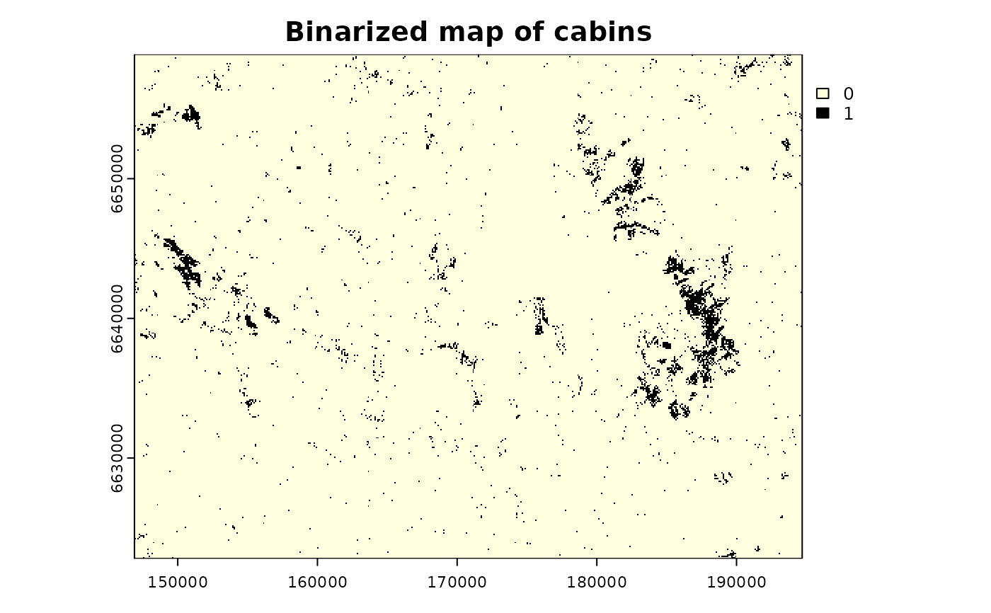
plot(cabins_bin, col = c("lightyellow", "black"),
main = "Binarized map of cabins")
#---
# define region in GRASS GIS
rgrass::execGRASS("g.region", raster = cabins_g,
flags = "p")
#> projection: 99 (unknown)
#> zone: 0
#> datum: etrs89
#> ellipsoid: grs80
#> north: 6658900
#> south: 6622800
#> west: 146900
#> east: 194700
#> nsres: 100
#> ewres: 100
#> rows: 361
#> cols: 478
#> cells: 172558
#---
# Guarantee input map is binary (zeros as background)
# Input map name within GRASS GIS - binary map
cabins_bin_g <- grass_binarize(cabins_g, breaks = 1, output = "cabins_example_bin",
null = 0, overwrite = TRUE)
#> Removing raster <inter_map>
# check input
cabins_bin <- rgrass::read_RAST("cabins_example_bin", return_format = "terra", NODATA = 255)
#> Checking GDAL data type and nodata value...
#> 2% 5% 8% 11% 14% 17% 20% 23% 26% 29% 32% 35% 38% 41% 44% 47% 50% 53% 56% 59% 62% 65% 68% 71% 74% 77% 80% 83% 86% 89% 92% 95% 98% 100%
#> Using GDAL data type <Byte>
#> Exporting raster data to RRASTER format...
#> 2% 5% 8% 11% 14% 17% 20% 23% 26% 29% 32% 35% 38% 41% 44% 47% 50% 53% 56% 59% 62% 65% 68% 71% 74% 77% 80% 83% 86% 89% 92% 95% 98% 100%
#> r.out.gdal complete. File </tmp/RtmpeYeIng/file27d6219c536c.grd> created.
plot(cabins_bin, col = c("lightyellow", "black"),
main = "Binarized map of cabins")
 #---
# Using 'r.mfilter' algorithm (default)
# Exponential decay
exp_name <- calc_zoi_cumulative(x = cabins_bin_g,
radius = 1000, zoi_limit = 0.01,
type = "exp_decay",
where = "GRASS",
g_overwrite = TRUE,
verbose = TRUE)
#> [1] "Calculating cumulative ZOI for 1000, shape exp_decay..."
#> 0% 3% 6% 9% 12% 15% 18% 21% 24% 27% 30% 33% 36% 39% 42% 45% 48% 51% 54% 57% 60% 63% 66% 69% 72% 75% 78% 81% 84% 87% 90% 93% 96% 99% 100%
#> Writing raster map <cabins_example_bin_zoi_cumulative_exp_decay1000>
# Bartlett decay
barlett_name <- calc_zoi_cumulative(x = cabins_bin_g,
radius = 1000,
type = "bartlett",
where = "GRASS",
g_overwrite = TRUE,
verbose = TRUE)
#> [1] "Calculating cumulative ZOI for 1000, shape bartlett..."
#> 0% 3% 6% 9% 12% 15% 18% 21% 24% 27% 30% 33% 36% 39% 42% 45% 48% 51% 54% 57% 60% 63% 66% 69% 72% 75% 78% 81% 84% 87% 90% 93% 96% 99% 100%
#> Writing raster map <cabins_example_bin_zoi_cumulative_bartlett1000>
# Gaussian decay
gauss_name <- calc_zoi_cumulative(x = cabins_bin_g,
radius = 1000, zoi_limit = 0.01,
type = "Gauss",
where = "GRASS",
g_overwrite = TRUE,
verbose = TRUE)
#> [1] "Calculating cumulative ZOI for 1000, shape Gauss..."
#> 0% 3% 6% 9% 12% 15% 18% 21% 24% 27% 30% 33% 36% 39% 42% 45% 48% 51% 54% 57% 60% 63% 66% 69% 72% 75% 78% 81% 84% 87% 90% 93% 96% 99% 100%
#> Writing raster map <cabins_example_bin_zoi_cumulative_Gauss1000>
# Threshold decay (circle, step)
threshold_name <- calc_zoi_cumulative(x = cabins_bin_g,
radius = 1000,
type = "threshold",
where = "GRASS",
g_overwrite = TRUE,
verbose = TRUE)
#> [1] "Calculating cumulative ZOI for 1000, shape threshold..."
#> 0% 3% 6% 9% 12% 15% 18% 21% 24% 27% 30% 33% 36% 39% 42% 45% 48% 51% 54% 57% 60% 63% 66% 69% 72% 75% 78% 81% 84% 87% 90% 93% 96% 99% 100%
#> Writing raster map <cabins_example_bin_zoi_cumulative_threshold1000>
(all_names <- c(exp_name, barlett_name, gauss_name, threshold_name))
#> [1] "cabins_example_bin_zoi_cumulative_exp_decay1000"
#> [2] "cabins_example_bin_zoi_cumulative_bartlett1000"
#> [3] "cabins_example_bin_zoi_cumulative_Gauss1000"
#> [4] "cabins_example_bin_zoi_cumulative_threshold1000"
# visualize
cabins_zoi_cumulative <- rgrass::read_RAST(all_names, return_format = "terra")
#> Checking GDAL data type and nodata value...
#> 2% 5% 8% 11% 14% 17% 20% 23% 26% 29% 32% 35% 38% 41% 44% 47% 50% 53% 56% 59% 62% 65% 68% 71% 74% 77% 80% 83% 86% 89% 92% 95% 98% 100%
#> Using GDAL data type <Float32>
#> Exporting raster data to RRASTER format...
#> 2% 5% 8% 11% 14% 17% 20% 23% 26% 29% 32% 35% 38% 41% 44% 47% 50% 53% 56% 59% 62% 65% 68% 71% 74% 77% 80% 83% 86% 89% 92% 95% 98% 100%
#> r.out.gdal complete. File </tmp/RtmpeYeIng/file27d6118a2233.grd> created.
#> Checking GDAL data type and nodata value...
#> 2% 5% 8% 11% 14% 17% 20% 23% 26% 29% 32% 35% 38% 41% 44% 47% 50% 53% 56% 59% 62% 65% 68% 71% 74% 77% 80% 83% 86% 89% 92% 95% 98% 100%
#> Using GDAL data type <Float32>
#> Exporting raster data to RRASTER format...
#> 2% 5% 8% 11% 14% 17% 20% 23% 26% 29% 32% 35% 38% 41% 44% 47% 50% 53% 56% 59% 62% 65% 68% 71% 74% 77% 80% 83% 86% 89% 92% 95% 98% 100%
#> r.out.gdal complete. File </tmp/RtmpeYeIng/file27d67ff92ba2.grd> created.
#> Checking GDAL data type and nodata value...
#> 2% 5% 8% 11% 14% 17% 20% 23% 26% 29% 32% 35% 38% 41% 44% 47% 50% 53% 56% 59% 62% 65% 68% 71% 74% 77% 80% 83% 86% 89% 92% 95% 98% 100%
#> Using GDAL data type <Float32>
#> Exporting raster data to RRASTER format...
#> 2% 5% 8% 11% 14% 17% 20% 23% 26% 29% 32% 35% 38% 41% 44% 47% 50% 53% 56% 59% 62% 65% 68% 71% 74% 77% 80% 83% 86% 89% 92% 95% 98% 100%
#> r.out.gdal complete. File </tmp/RtmpeYeIng/file27d66821a1ee.grd> created.
#> Checking GDAL data type and nodata value...
#> 2% 5% 8% 11% 14% 17% 20% 23% 26% 29% 32% 35% 38% 41% 44% 47% 50% 53% 56% 59% 62% 65% 68% 71% 74% 77% 80% 83% 86% 89% 92% 95% 98% 100%
#> Using GDAL data type <Float32>
#> Exporting raster data to RRASTER format...
#> 2% 5% 8% 11% 14% 17% 20% 23% 26% 29% 32% 35% 38% 41% 44% 47% 50% 53% 56% 59% 62% 65% 68% 71% 74% 77% 80% 83% 86% 89% 92% 95% 98% 100%
#> r.out.gdal complete. File </tmp/RtmpeYeIng/file27d64ea787e7.grd> created.
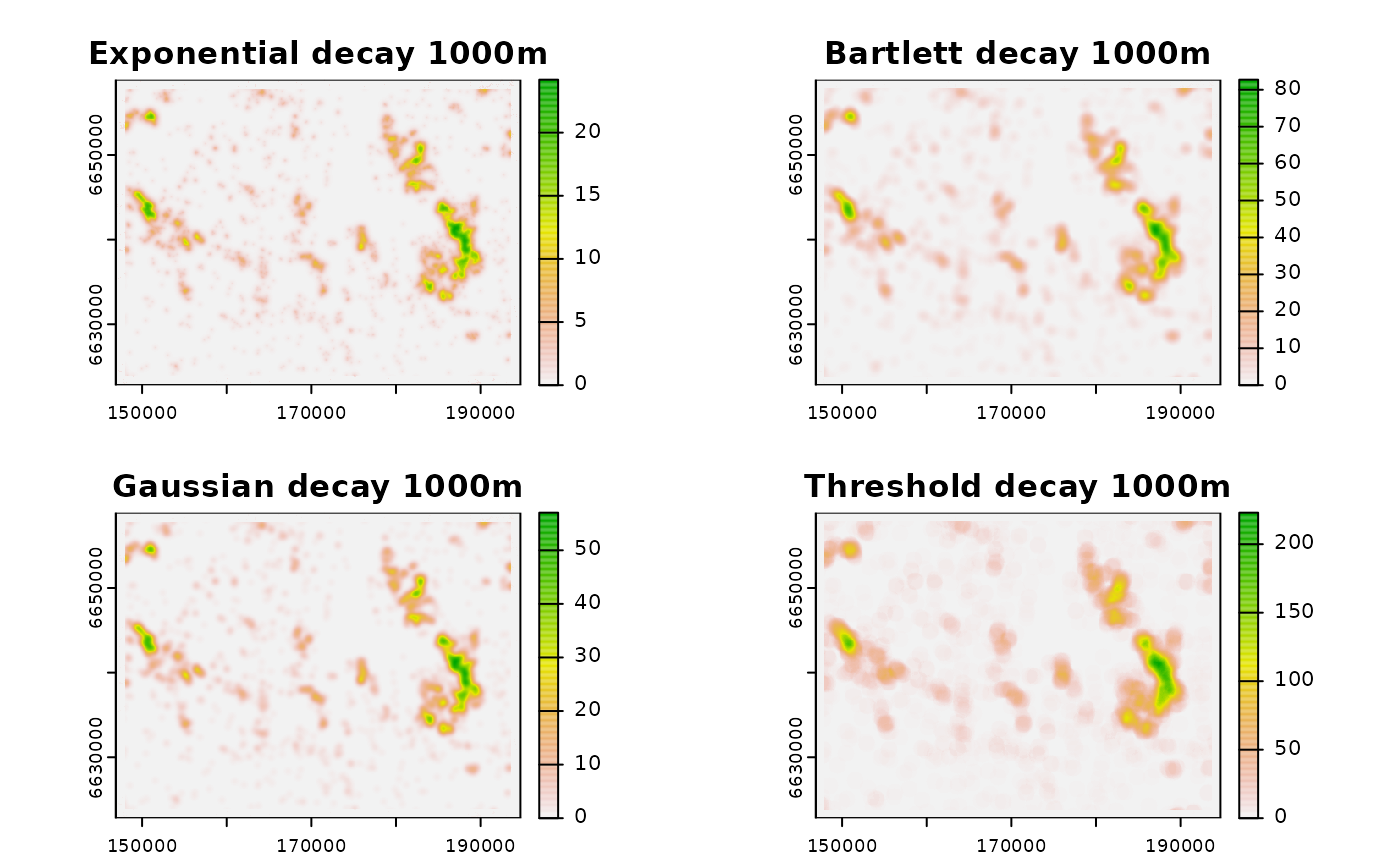
title_plot <- c("Exponential decay 1000m", "Bartlett decay 1000m",
"Gaussian decay 1000m", "Threshold decay 1000m")
terra::plot(cabins_zoi_cumulative, main = title_plot)
#---
# Using 'r.mfilter' algorithm (default)
# Exponential decay
exp_name <- calc_zoi_cumulative(x = cabins_bin_g,
radius = 1000, zoi_limit = 0.01,
type = "exp_decay",
where = "GRASS",
g_overwrite = TRUE,
verbose = TRUE)
#> [1] "Calculating cumulative ZOI for 1000, shape exp_decay..."
#> 0% 3% 6% 9% 12% 15% 18% 21% 24% 27% 30% 33% 36% 39% 42% 45% 48% 51% 54% 57% 60% 63% 66% 69% 72% 75% 78% 81% 84% 87% 90% 93% 96% 99% 100%
#> Writing raster map <cabins_example_bin_zoi_cumulative_exp_decay1000>
# Bartlett decay
barlett_name <- calc_zoi_cumulative(x = cabins_bin_g,
radius = 1000,
type = "bartlett",
where = "GRASS",
g_overwrite = TRUE,
verbose = TRUE)
#> [1] "Calculating cumulative ZOI for 1000, shape bartlett..."
#> 0% 3% 6% 9% 12% 15% 18% 21% 24% 27% 30% 33% 36% 39% 42% 45% 48% 51% 54% 57% 60% 63% 66% 69% 72% 75% 78% 81% 84% 87% 90% 93% 96% 99% 100%
#> Writing raster map <cabins_example_bin_zoi_cumulative_bartlett1000>
# Gaussian decay
gauss_name <- calc_zoi_cumulative(x = cabins_bin_g,
radius = 1000, zoi_limit = 0.01,
type = "Gauss",
where = "GRASS",
g_overwrite = TRUE,
verbose = TRUE)
#> [1] "Calculating cumulative ZOI for 1000, shape Gauss..."
#> 0% 3% 6% 9% 12% 15% 18% 21% 24% 27% 30% 33% 36% 39% 42% 45% 48% 51% 54% 57% 60% 63% 66% 69% 72% 75% 78% 81% 84% 87% 90% 93% 96% 99% 100%
#> Writing raster map <cabins_example_bin_zoi_cumulative_Gauss1000>
# Threshold decay (circle, step)
threshold_name <- calc_zoi_cumulative(x = cabins_bin_g,
radius = 1000,
type = "threshold",
where = "GRASS",
g_overwrite = TRUE,
verbose = TRUE)
#> [1] "Calculating cumulative ZOI for 1000, shape threshold..."
#> 0% 3% 6% 9% 12% 15% 18% 21% 24% 27% 30% 33% 36% 39% 42% 45% 48% 51% 54% 57% 60% 63% 66% 69% 72% 75% 78% 81% 84% 87% 90% 93% 96% 99% 100%
#> Writing raster map <cabins_example_bin_zoi_cumulative_threshold1000>
(all_names <- c(exp_name, barlett_name, gauss_name, threshold_name))
#> [1] "cabins_example_bin_zoi_cumulative_exp_decay1000"
#> [2] "cabins_example_bin_zoi_cumulative_bartlett1000"
#> [3] "cabins_example_bin_zoi_cumulative_Gauss1000"
#> [4] "cabins_example_bin_zoi_cumulative_threshold1000"
# visualize
cabins_zoi_cumulative <- rgrass::read_RAST(all_names, return_format = "terra")
#> Checking GDAL data type and nodata value...
#> 2% 5% 8% 11% 14% 17% 20% 23% 26% 29% 32% 35% 38% 41% 44% 47% 50% 53% 56% 59% 62% 65% 68% 71% 74% 77% 80% 83% 86% 89% 92% 95% 98% 100%
#> Using GDAL data type <Float32>
#> Exporting raster data to RRASTER format...
#> 2% 5% 8% 11% 14% 17% 20% 23% 26% 29% 32% 35% 38% 41% 44% 47% 50% 53% 56% 59% 62% 65% 68% 71% 74% 77% 80% 83% 86% 89% 92% 95% 98% 100%
#> r.out.gdal complete. File </tmp/RtmpeYeIng/file27d6118a2233.grd> created.
#> Checking GDAL data type and nodata value...
#> 2% 5% 8% 11% 14% 17% 20% 23% 26% 29% 32% 35% 38% 41% 44% 47% 50% 53% 56% 59% 62% 65% 68% 71% 74% 77% 80% 83% 86% 89% 92% 95% 98% 100%
#> Using GDAL data type <Float32>
#> Exporting raster data to RRASTER format...
#> 2% 5% 8% 11% 14% 17% 20% 23% 26% 29% 32% 35% 38% 41% 44% 47% 50% 53% 56% 59% 62% 65% 68% 71% 74% 77% 80% 83% 86% 89% 92% 95% 98% 100%
#> r.out.gdal complete. File </tmp/RtmpeYeIng/file27d67ff92ba2.grd> created.
#> Checking GDAL data type and nodata value...
#> 2% 5% 8% 11% 14% 17% 20% 23% 26% 29% 32% 35% 38% 41% 44% 47% 50% 53% 56% 59% 62% 65% 68% 71% 74% 77% 80% 83% 86% 89% 92% 95% 98% 100%
#> Using GDAL data type <Float32>
#> Exporting raster data to RRASTER format...
#> 2% 5% 8% 11% 14% 17% 20% 23% 26% 29% 32% 35% 38% 41% 44% 47% 50% 53% 56% 59% 62% 65% 68% 71% 74% 77% 80% 83% 86% 89% 92% 95% 98% 100%
#> r.out.gdal complete. File </tmp/RtmpeYeIng/file27d66821a1ee.grd> created.
#> Checking GDAL data type and nodata value...
#> 2% 5% 8% 11% 14% 17% 20% 23% 26% 29% 32% 35% 38% 41% 44% 47% 50% 53% 56% 59% 62% 65% 68% 71% 74% 77% 80% 83% 86% 89% 92% 95% 98% 100%
#> Using GDAL data type <Float32>
#> Exporting raster data to RRASTER format...
#> 2% 5% 8% 11% 14% 17% 20% 23% 26% 29% 32% 35% 38% 41% 44% 47% 50% 53% 56% 59% 62% 65% 68% 71% 74% 77% 80% 83% 86% 89% 92% 95% 98% 100%
#> r.out.gdal complete. File </tmp/RtmpeYeIng/file27d64ea787e7.grd> created.
title_plot <- c("Exponential decay 1000m", "Bartlett decay 1000m",
"Gaussian decay 1000m", "Threshold decay 1000m")
terra::plot(cabins_zoi_cumulative, main = title_plot)
 #---
# calculate density vs cumulative ZoI
exp_name_d <- calc_zoi_cumulative(x = cabins_bin_g,
radius = 1000, zoi_limit = 0.01,
type = "exp_decay", output_type = "density",
where = "GRASS",
g_overwrite = TRUE,
verbose = TRUE)
#> [1] "Calculating density for 1000, shape exp_decay..."
#> 0% 3% 6% 9% 12% 15% 18% 21% 24% 27% 30% 33% 36% 39% 42% 45% 48% 51% 54% 57% 60% 63% 66% 69% 72% 75% 78% 81% 84% 87% 90% 93% 96% 99% 100%
#> Writing raster map <cabins_example_bin_density_exp_decay1000>
cabins_density <- rgrass::read_RAST(exp_name_d, return_format = "terra")
#> Checking GDAL data type and nodata value...
#> 2% 5% 8% 11% 14% 17% 20% 23% 26% 29% 32% 35% 38% 41% 44% 47% 50% 53% 56% 59% 62% 65% 68% 71% 74% 77% 80% 83% 86% 89% 92% 95% 98% 100%
#> Using GDAL data type <Float32>
#> Exporting raster data to RRASTER format...
#> 2% 5% 8% 11% 14% 17% 20% 23% 26% 29% 32% 35% 38% 41% 44% 47% 50% 53% 56% 59% 62% 65% 68% 71% 74% 77% 80% 83% 86% 89% 92% 95% 98% 100%
#> r.out.gdal complete. File </tmp/RtmpeYeIng/file27d645ae0ad8.grd> created.
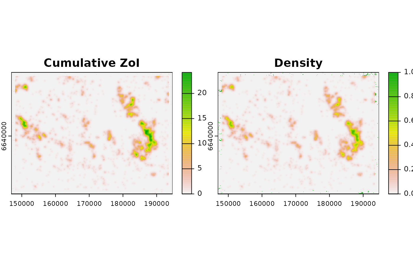
terra::plot(c(cabins_zoi_cumulative[[1]], cabins_density),
main = c("Cumulative ZoI", "Density"))
#---
# calculate density vs cumulative ZoI
exp_name_d <- calc_zoi_cumulative(x = cabins_bin_g,
radius = 1000, zoi_limit = 0.01,
type = "exp_decay", output_type = "density",
where = "GRASS",
g_overwrite = TRUE,
verbose = TRUE)
#> [1] "Calculating density for 1000, shape exp_decay..."
#> 0% 3% 6% 9% 12% 15% 18% 21% 24% 27% 30% 33% 36% 39% 42% 45% 48% 51% 54% 57% 60% 63% 66% 69% 72% 75% 78% 81% 84% 87% 90% 93% 96% 99% 100%
#> Writing raster map <cabins_example_bin_density_exp_decay1000>
cabins_density <- rgrass::read_RAST(exp_name_d, return_format = "terra")
#> Checking GDAL data type and nodata value...
#> 2% 5% 8% 11% 14% 17% 20% 23% 26% 29% 32% 35% 38% 41% 44% 47% 50% 53% 56% 59% 62% 65% 68% 71% 74% 77% 80% 83% 86% 89% 92% 95% 98% 100%
#> Using GDAL data type <Float32>
#> Exporting raster data to RRASTER format...
#> 2% 5% 8% 11% 14% 17% 20% 23% 26% 29% 32% 35% 38% 41% 44% 47% 50% 53% 56% 59% 62% 65% 68% 71% 74% 77% 80% 83% 86% 89% 92% 95% 98% 100%
#> r.out.gdal complete. File </tmp/RtmpeYeIng/file27d645ae0ad8.grd> created.
terra::plot(c(cabins_zoi_cumulative[[1]], cabins_density),
main = c("Cumulative ZoI", "Density"))
 #---
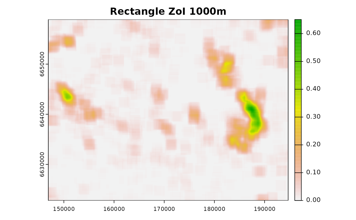
# Using 'r.resamp.filter' algorithm
# rectangle
rectangle_resamp_filt <- calc_zoi_cumulative(x = cabins_bin_g,
radius = 1000,
type = "box",
output_type = "density",
where = "GRASS",
g_module = "r.resamp.filter",
g_overwrite = TRUE,
verbose = TRUE)
#> [1] "Calculating density for 1000, shape box..."
#> 0% 3% 6% 9% 12% 15% 18% 21% 24% 27% 30% 33% 36% 39% 42% 45% 48% 51% 54% 57% 60% 63% 66% 69% 72% 75% 78% 81% 84% 87% 90% 93% 96% 99% 100%
rgrass::read_RAST(rectangle_resamp_filt, return_format = "terra") |>
plot(main = "Rectangle ZoI 1000m")
#> Checking GDAL data type and nodata value...
#> 2% 5% 8% 11% 14% 17% 20% 23% 26% 29% 32% 35% 38% 41% 44% 47% 50% 53% 56% 59% 62% 65% 68% 71% 74% 77% 80% 83% 86% 89% 92% 95% 98% 100%
#> Using GDAL data type <Float64>
#> Exporting raster data to RRASTER format...
#> 2% 5% 8% 11% 14% 17% 20% 23% 26% 29% 32% 35% 38% 41% 44% 47% 50% 53% 56% 59% 62% 65% 68% 71% 74% 77% 80% 83% 86% 89% 92% 95% 98% 100%
#> r.out.gdal complete. File </tmp/RtmpeYeIng/file27d6525a5f5e.grd> created.
#---
# Using 'r.resamp.filter' algorithm
# rectangle
rectangle_resamp_filt <- calc_zoi_cumulative(x = cabins_bin_g,
radius = 1000,
type = "box",
output_type = "density",
where = "GRASS",
g_module = "r.resamp.filter",
g_overwrite = TRUE,
verbose = TRUE)
#> [1] "Calculating density for 1000, shape box..."
#> 0% 3% 6% 9% 12% 15% 18% 21% 24% 27% 30% 33% 36% 39% 42% 45% 48% 51% 54% 57% 60% 63% 66% 69% 72% 75% 78% 81% 84% 87% 90% 93% 96% 99% 100%
rgrass::read_RAST(rectangle_resamp_filt, return_format = "terra") |>
plot(main = "Rectangle ZoI 1000m")
#> Checking GDAL data type and nodata value...
#> 2% 5% 8% 11% 14% 17% 20% 23% 26% 29% 32% 35% 38% 41% 44% 47% 50% 53% 56% 59% 62% 65% 68% 71% 74% 77% 80% 83% 86% 89% 92% 95% 98% 100%
#> Using GDAL data type <Float64>
#> Exporting raster data to RRASTER format...
#> 2% 5% 8% 11% 14% 17% 20% 23% 26% 29% 32% 35% 38% 41% 44% 47% 50% 53% 56% 59% 62% 65% 68% 71% 74% 77% 80% 83% 86% 89% 92% 95% 98% 100%
#> r.out.gdal complete. File </tmp/RtmpeYeIng/file27d6525a5f5e.grd> created.
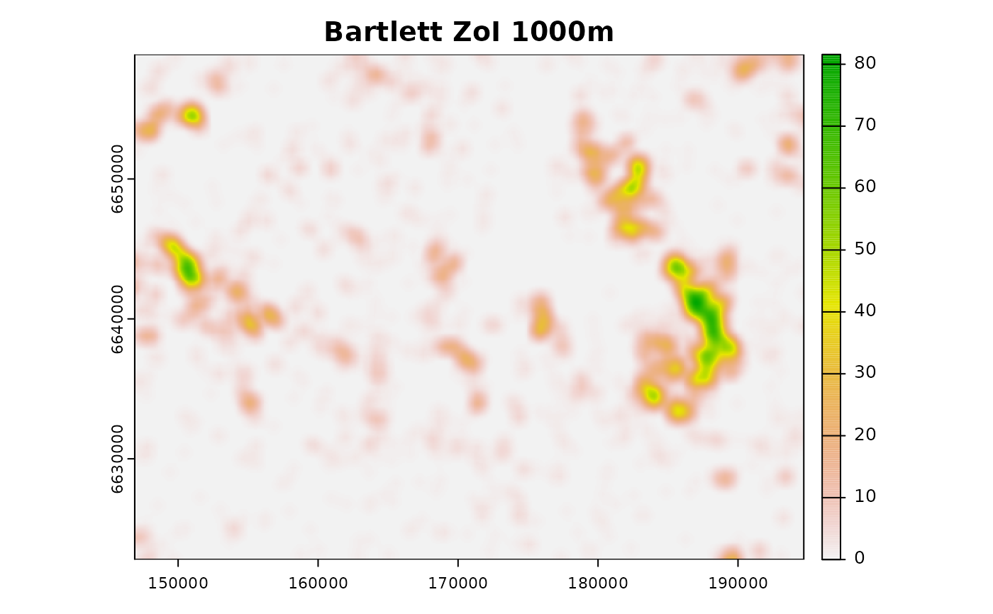
 # bartlett
bartlett_resamp_filt <- calc_zoi_cumulative(x = cabins_bin_g,
radius = 1000,
type = "bartlett",
output_type = "cumulative_zoi",
where = "GRASS",
g_module = "r.resamp.filter",
g_overwrite = TRUE,
verbose = TRUE)
#> [1] "Calculating cumulative ZOI for 1000, shape bartlett..."
#> 0% 3% 6% 9% 12% 15% 18% 21% 24% 27% 30% 33% 36% 39% 42% 45% 48% 51% 54% 57% 60% 63% 66% 69% 72% 75% 78% 81% 84% 87% 90% 93% 96% 99% 100%
#> [1] "Rescaling from density to cumulative ZOI..."
#> [1] "cabins_example_bin_zoi_cumulative_bartlett1000 = cabins_example_bin_zoi_cumulative_bartlett1000_temp/0.0095562598354124"
#> Removing raster <cabins_example_bin_zoi_cumulative_bartlett1000_temp>
rgrass::read_RAST(bartlett_resamp_filt, return_format = "terra") |>
plot(main = "Bartlett ZoI 1000m")
#> Checking GDAL data type and nodata value...
#> 2% 5% 8% 11% 14% 17% 20% 23% 26% 29% 32% 35% 38% 41% 44% 47% 50% 53% 56% 59% 62% 65% 68% 71% 74% 77% 80% 83% 86% 89% 92% 95% 98% 100%
#> Using GDAL data type <Float64>
#> Exporting raster data to RRASTER format...
#> 2% 5% 8% 11% 14% 17% 20% 23% 26% 29% 32% 35% 38% 41% 44% 47% 50% 53% 56% 59% 62% 65% 68% 71% 74% 77% 80% 83% 86% 89% 92% 95% 98% 100%
#> r.out.gdal complete. File </tmp/RtmpeYeIng/file27d6e679d30.grd> created.
# bartlett
bartlett_resamp_filt <- calc_zoi_cumulative(x = cabins_bin_g,
radius = 1000,
type = "bartlett",
output_type = "cumulative_zoi",
where = "GRASS",
g_module = "r.resamp.filter",
g_overwrite = TRUE,
verbose = TRUE)
#> [1] "Calculating cumulative ZOI for 1000, shape bartlett..."
#> 0% 3% 6% 9% 12% 15% 18% 21% 24% 27% 30% 33% 36% 39% 42% 45% 48% 51% 54% 57% 60% 63% 66% 69% 72% 75% 78% 81% 84% 87% 90% 93% 96% 99% 100%
#> [1] "Rescaling from density to cumulative ZOI..."
#> [1] "cabins_example_bin_zoi_cumulative_bartlett1000 = cabins_example_bin_zoi_cumulative_bartlett1000_temp/0.0095562598354124"
#> Removing raster <cabins_example_bin_zoi_cumulative_bartlett1000_temp>
rgrass::read_RAST(bartlett_resamp_filt, return_format = "terra") |>
plot(main = "Bartlett ZoI 1000m")
#> Checking GDAL data type and nodata value...
#> 2% 5% 8% 11% 14% 17% 20% 23% 26% 29% 32% 35% 38% 41% 44% 47% 50% 53% 56% 59% 62% 65% 68% 71% 74% 77% 80% 83% 86% 89% 92% 95% 98% 100%
#> Using GDAL data type <Float64>
#> Exporting raster data to RRASTER format...
#> 2% 5% 8% 11% 14% 17% 20% 23% 26% 29% 32% 35% 38% 41% 44% 47% 50% 53% 56% 59% 62% 65% 68% 71% 74% 77% 80% 83% 86% 89% 92% 95% 98% 100%
#> r.out.gdal complete. File </tmp/RtmpeYeIng/file27d6e679d30.grd> created.
 # not run
# Gaussian - to be implemented!
if (FALSE) { # \dontrun{
gauss_resamp_filt <- calc_zoi_cumulative(x = cabins_bin_g,
radius = "1000,3000",
type = "gauss,box",
output_type = "cumulative_zoi",
where = "GRASS",
module = "r.resamp.filter",
overwrite = TRUE, quiet = FALSE)
rgrass::read_RAST(bartlett_resamp_filt, return_format = "terra") |>
plot()
} # }
# remove rasters created
# to_remove_rast <- unique(c(all_names, exp_name_d,
# rectangle_resamp_filt, bartlett_resamp_filt))
# rgrass::execGRASS("g.remove", type = "vect", name = to_remove_vect, flags = "f")
# rgrass::execGRASS("g.remove", type = "rast", name = to_remove_rast, flags = "f")
# not run
# Gaussian - to be implemented!
if (FALSE) { # \dontrun{
gauss_resamp_filt <- calc_zoi_cumulative(x = cabins_bin_g,
radius = "1000,3000",
type = "gauss,box",
output_type = "cumulative_zoi",
where = "GRASS",
module = "r.resamp.filter",
overwrite = TRUE, quiet = FALSE)
rgrass::read_RAST(bartlett_resamp_filt, return_format = "terra") |>
plot()
} # }
# remove rasters created
# to_remove_rast <- unique(c(all_names, exp_name_d,
# rectangle_resamp_filt, bartlett_resamp_filt))
# rgrass::execGRASS("g.remove", type = "vect", name = to_remove_vect, flags = "f")
# rgrass::execGRASS("g.remove", type = "rast", name = to_remove_rast, flags = "f")