This function predicts and plots response curves from a bag of models while
varying one or more focal predictors in dfvar. Non-focal predictors are kept
at baseline values. It supports confidence intervals from weighted quantiles
and optional individual-model predictions.
Usage
plot_response(
  x,
  dfvar,
  data,
  type = c("linear", "exponential", "logit", "cloglog")[1],
  zoi_shape = c("exp_decay", "gaussian_decay", "linear_decay", "threshold_decay")[1],
  which_cumulative = "cumulative",
  ci = TRUE,
  indiv_pred = FALSE,
  wq_probs = c(0.025, 0.5, 0.975),
  baseline = c("median", "mean", "zero")[1],
  zoi = FALSE,
  type_feature = c("point", "line", "area")[1],
  type_feature_recompute = FALSE,
  zoi_limit = 0.05,
  resolution = 100,
  line_value = 1,
  plot_mean = TRUE,
  plot_median = TRUE,
  n_features = 1,
  normalize = c(FALSE, "mean", "median", "ci")[1],
  logx = FALSE,
  ylim = NULL,
  y_lab = "Relative Selection Strength",
  col_ci = "grey",
  col_indiv = "grey",
  col_mean = "black",
  col_median = "red",
  linewidth_indiv = 1.2,
  linewidth_mean = 1.2,
  linewidth_median = 1.2,
  alpha_ci = 0.5,
  alpha_indiv = 0.3
)

# S3 method for class 'bag'
plot_response(
  x,
  dfvar,
  data,
  type = c("linear", "exponential", "logit", "cloglog")[1],
  zoi_shape = c("exp_decay", "gaussian_decay", "linear_decay", "threshold_decay")[1],
  which_cumulative = "cumulative",
  ci = TRUE,
  indiv_pred = FALSE,
  wq_probs = c(0.025, 0.5, 0.975),
  baseline = c("median", "mean", "zero")[1],
  zoi = FALSE,
  type_feature = c("point", "line", "area")[1],
  type_feature_recompute = FALSE,
  zoi_limit = 0.05,
  resolution = 100,
  line_value = 1,
  ggplot = T,
  plot_mean = TRUE,
  plot_median = TRUE,
  n_features = 1,
  normalize = c(FALSE, "mean", "median", "ci")[1],
  logx = FALSE,
  ylim = NULL,
  y_lab = "Relative Selection Strength",
  col_ci = "grey",
  col_indiv = "grey",
  col_mean = "black",
  col_median = "red",
  linewidth_indiv = 1.2,
  linewidth_mean = 1.2,
  linewidth_median = 1.2,
  alpha_ci = 0.5,
  alpha_indiv = 0.3
)
Arguments
- x
[bag,list]
A bag of models created withbag_models().- dfvar
[data.frame]
Data frame with values of focal predictors to vary and predict over. The column names of thedata.framemight correspond exactly to the model covariates or to parts of that (for instance, "roads_paved_" to refer to all ZOI variables related to paved roads).- data
[data.frame]
Original data used for model fitting. Used only for taking the categories of the categorical variables. Irrelevant if there is no categorical variables.- type
[character(1)="linear"]{"linear", "exponential", "logit", "cloglog"}
Prediction scale.- zoi_shape
[character(1)="exp_decay"]{"exp_decay", "gaussian_decay", "linear_decay", "threshold_decay"}
ZOI decay shape used whenzoi = TRUE.- which_cumulative
[character(1)="cumulative"]
Pattern used to identify cumulative ZOI terms.- ci
[logical(1)=TRUE]
IfTRUE(default), plot weighted confidence intervals usingwq_probs.- indiv_pred
[logical(1)=FALSE]
IfTRUE, include curves from individual models (only models with positive weight).- wq_probs
[numeric,vector=c(0.025, 0.5, 0.975)]
Weighted quantile probabilities used for confidence intervals and median.- baseline
[character(1)="median"]{"median", "mean", "zero"}
Baseline value strategy for non-focal predictors. Variable are either kept constant at the mean or median values, or left as zero. Categorical variables are set to their reference level, retrieved fromdata.- zoi
[logical(1)=FALSE]
IfTRUE, variables values indfvarare interpreted as distance from a disturbance source, to be transformed into ZOI predictors.- type_feature
[character(1)="point"]{"point", "line", "area"}
Feature type for ZOI prediction.- type_feature_recompute
[logical(1)=FALSE]
IfTRUE, recompute line- or area-feature raster representation for ZOI calculations.- zoi_limit
[numeric(1)=0.05]
Lower influence threshold used by non-vanishing ZOI functions. Seezoi_functions().- resolution
[numeric(1)=100]
Raster resolution used for line-feature ZOI approximation. Used when recomputing the ZOI variables for line and area features.- line_value
[numeric(1)=1]
Value assigned to line raster cells whentype_feature = "line". Used when recomputing the ZOI variables for line and area features.- plot_mean
[logical(1)=TRUE]
Plot weighted mean response line.- plot_median
[logical(1)=TRUE]
Plot weighted median response line.- n_features
[numeric(1)=1]
Number of features used in ZOI prediction. To represent the cumulative impact of multiple features, usen_features > 1.- normalize
[logical or character]
Optional y-axis normalization: one ofFALSE,"mean","median", or"ci". Default isFALSE, which assumes no normalization.- logx
[logical(1)=FALSE]
IfTRUE, use log10 scaling on x-axis.- ylim
[NULL or ggplot2 scale/coord limits]
Optional y-axis limits.- y_lab
[character(1)="Relative Selection Strength"]
Y-axis label.- col_ci
[character(1)="grey"]
Fill color for confidence ribbon.- col_indiv
[character(1)="grey"]
Color for individual model lines.- col_mean
[character(1)="black"]
Color for weighted mean line.- col_median
[character(1)="red"]
Color for weighted median line.- linewidth_indiv
[numeric(1)=1.2]
Line width for individual model lines.- linewidth_mean
[numeric(1)=1.2]
Line width for weighted mean line.- linewidth_median
[numeric(1)=1.2]
Line width for weighted median line.- alpha_ci
[numeric(1)=0.5]
Alpha transparency for confidence ribbon.- alpha_indiv
[numeric(1)=0.3]
Alpha transparency for individual model lines.- ggplot
[logical(1)=TRUE]
IfTRUE, return a ggplot object; otherwise return a prediction data frame.
Value
If ggplot = TRUE, a ggplot object with response curves.
If ggplot = FALSE, a data frame with dfvar, summary predictions, and
optionally individual-model predictions when indiv_pred = TRUE.
Examples
#---
# fit a bag to be tested
# load packages
library(glmnet)
library(ggplot2)
# load data
data("reindeer_rsf")
# rename it just for convenience
dat <- reindeer_rsf
# formula initial structure
f <- use ~ private_cabins_XXX + public_cabins_high_XXX +
trails_XXX +
NORUTreclass +
# poly(norway_pca_klima_axis1, 2, raw = TRUE) +
# poly(norway_pca_klima_axis2, 2, raw = TRUE) +
norway_pca_klima_axis1 + norway_pca_klima_axis1_sq +
norway_pca_klima_axis2 + norway_pca_klima_axis2_sq +
norway_pca_klima_axis3 + norway_pca_klima_axis4
# add ZOI terms to the formula
zois <- c(100, 250, 500, 1000, 2500, 5000, 10000, 20000)
f <- add_zoi_formula(f, zoi_radius = zois, pattern = "XXX",
type = c("cumulative_exp_decay"),
separator = "", predictor_table = TRUE)$formula
# sampling - random sampling
set.seed(1234)
samples <- create_resamples(y = dat$use,
p = c(0.2, 0.2, 0.2),
times = 10,
colH0 = NULL)
#> [1] "Starting random sampling..."
# fit multiple models
fittedl <- bag_fit_net_logit(f,
data = dat,
samples = samples,
standardize = "internal", # glmnet does the standardization of covariates
metric = "AUC",
method = "AdaptiveLasso",
parallel = "mclapply",
mc.cores = 2)
# bag models in a single object
bag_object <- bag_models(fittedl, dat, score_threshold = 0.7)
#---
# plot predictions for non-ZOI variables
# plot for PCA1
dfvar <- data.frame(norway_pca_klima_axis1 = seq(min(bag_object$data_summary$norway_pca_klima_axis1),
max(bag_object$data_summary$norway_pca_klima_axis1),
length.out = 100))
dfvar$norway_pca_klima_axis1_sq = dfvar$norway_pca_klima_axis1**2
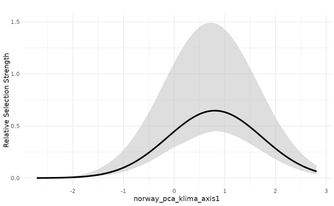
# plot mean response in linear scale with weighted interquartile range
plot_response(bag_object,
dfvar = dfvar,
data = dat,
wq_probs = c(0.25, 0.5, 0.75),
plot_median = FALSE) # remove median, plot only weighted mean
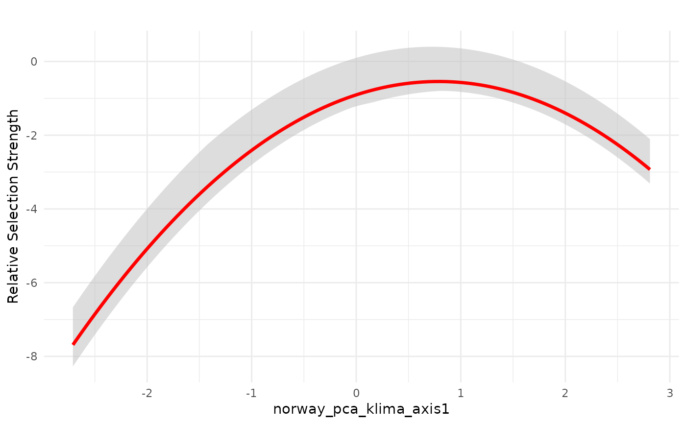 # plot median response in exponential scale with weighted interquartile range
plot_response(bag_object,
dfvar = dfvar,
data = dat,
type = "exp",
wq_probs = c(0.25, 0.5, 0.75),
plot_mean = FALSE) # remove mean, plot only weighted median
# plot median response in exponential scale with weighted interquartile range
plot_response(bag_object,
dfvar = dfvar,
data = dat,
type = "exp",
wq_probs = c(0.25, 0.5, 0.75),
plot_mean = FALSE) # remove mean, plot only weighted median
 #---
# plot predictions for ZOI variables
# plot for private cabins
# define newdata based only on the distances from the source (public cabins)
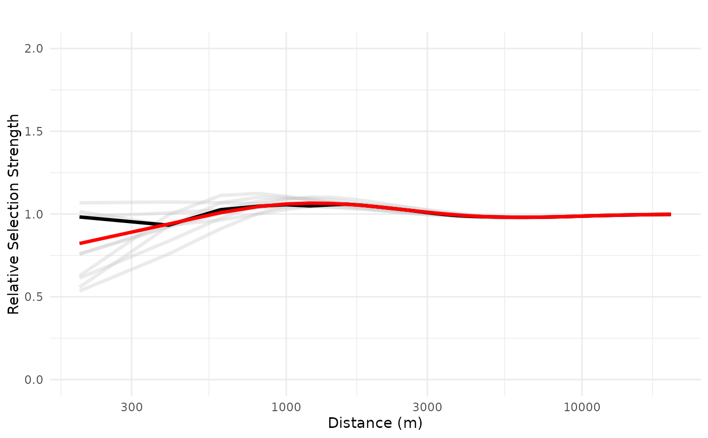
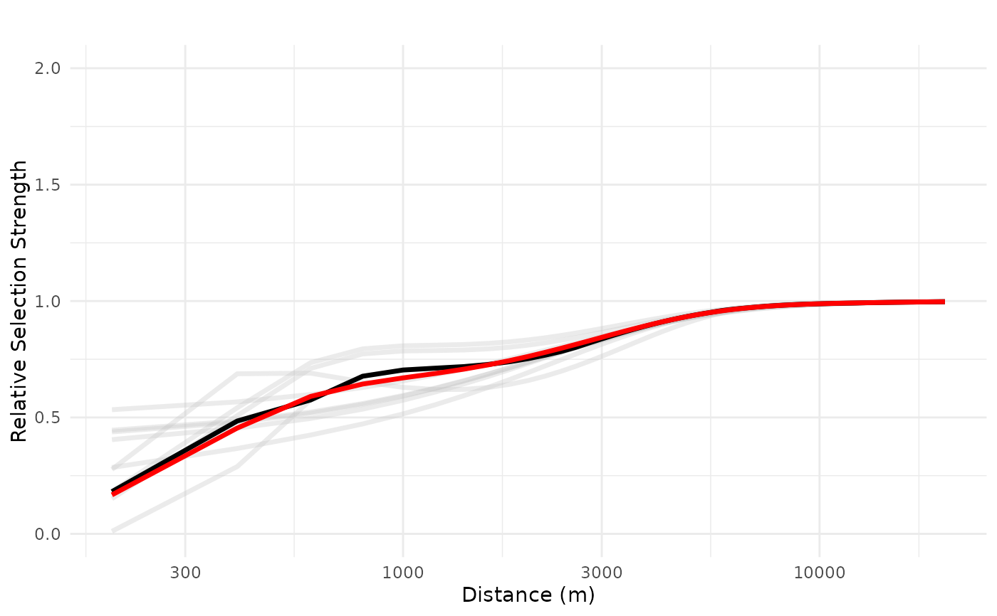
dfvar = data.frame(private_cabins = 1e3*seq(0.2, 20, length.out = 100))
# plot mean response in exponential scale, with individual lines, x in log scale
# in exponential scale, relative selection strength = 1 corresponse to no effect
# prediction for for 1 cabin only
plot_response(bag_object,
dfvar = dfvar,
data = dat,
type = "exp",
zoi = TRUE,
ci = FALSE,
indiv_pred = TRUE,
logx = TRUE,
ylim = ylim(0, 2))
#---
# plot predictions for ZOI variables
# plot for private cabins
# define newdata based only on the distances from the source (public cabins)
dfvar = data.frame(private_cabins = 1e3*seq(0.2, 20, length.out = 100))
# plot mean response in exponential scale, with individual lines, x in log scale
# in exponential scale, relative selection strength = 1 corresponse to no effect
# prediction for for 1 cabin only
plot_response(bag_object,
dfvar = dfvar,
data = dat,
type = "exp",
zoi = TRUE,
ci = FALSE,
indiv_pred = TRUE,
logx = TRUE,
ylim = ylim(0, 2))
 # prediction for for 10 cabins located at the origin
plot_response(bag_object,
dfvar = dfvar,
data = dat,
type = "exp",
zoi = TRUE,
n_features = 10,
ci = FALSE,
indiv_pred = TRUE,
logx = TRUE,
ylim = ylim(0, 2))
# prediction for for 10 cabins located at the origin
plot_response(bag_object,
dfvar = dfvar,
data = dat,
type = "exp",
zoi = TRUE,
n_features = 10,
ci = FALSE,
indiv_pred = TRUE,
logx = TRUE,
ylim = ylim(0, 2))
 #---
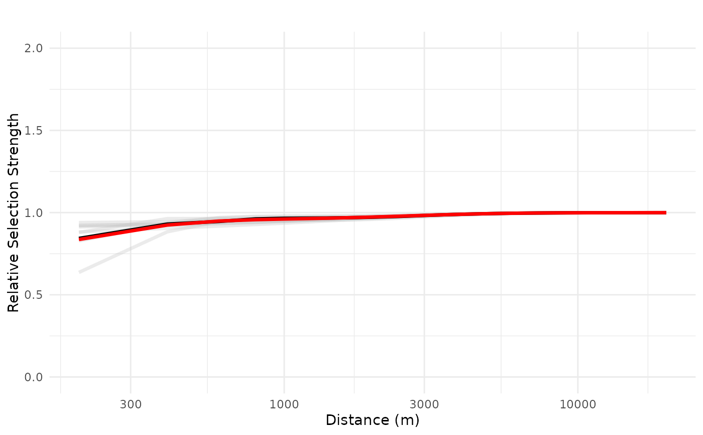
# plot predictions for linear ZOI variables
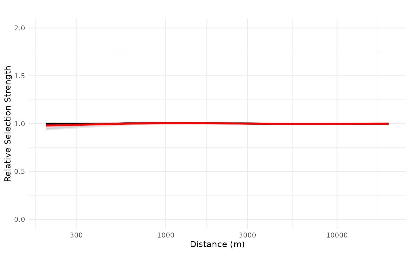
# plot for tourist trails
# define newdata based only on the distances from the source (public cabins)
dfvar = data.frame(trails = 1e3*seq(0.2, 20, length.out = 100))
# plot mean response in exponential scale, with individual lines, x in log scale
# in exponential scale, relative selection strength = 1 corresponse to no effect
# prediction for for 1 cabin only
plot_response(bag_object,
dfvar = dfvar,
data = dat,
type = "exp",
zoi = TRUE,
ci = FALSE,
indiv_pred = TRUE,
logx = TRUE,
ylim = ylim(0, 2))
#---
# plot predictions for linear ZOI variables
# plot for tourist trails
# define newdata based only on the distances from the source (public cabins)
dfvar = data.frame(trails = 1e3*seq(0.2, 20, length.out = 100))
# plot mean response in exponential scale, with individual lines, x in log scale
# in exponential scale, relative selection strength = 1 corresponse to no effect
# prediction for for 1 cabin only
plot_response(bag_object,
dfvar = dfvar,
data = dat,
type = "exp",
zoi = TRUE,
ci = FALSE,
indiv_pred = TRUE,
logx = TRUE,
ylim = ylim(0, 2))
 # prediction for for 10 cabins located at the origin
plot_response(bag_object,
dfvar = dfvar,
data = dat,
type = "exp",
zoi = TRUE,
n_features = 10,
ci = FALSE,
indiv_pred = TRUE,
logx = TRUE,
ylim = ylim(0, 2))
# prediction for for 10 cabins located at the origin
plot_response(bag_object,
dfvar = dfvar,
data = dat,
type = "exp",
zoi = TRUE,
n_features = 10,
ci = FALSE,
indiv_pred = TRUE,
logx = TRUE,
ylim = ylim(0, 2))