2  Study area and trenching data

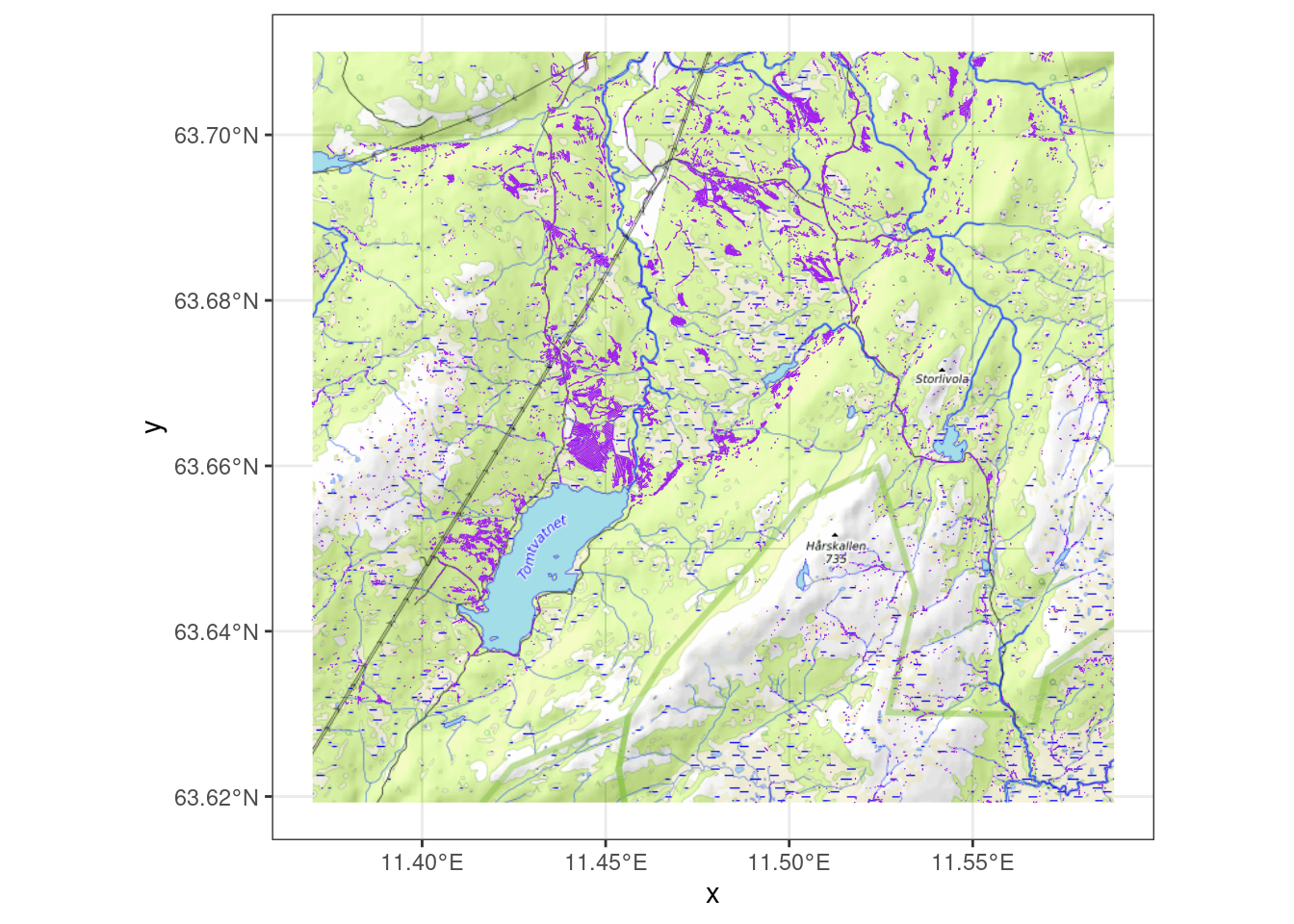
In this project we will use data from Levanger in central Norway. This area was part of the pilot study to identify mire trenches in Norway based on LiDAR (Jansson et al. 2024) (see also Chapter 1).

path <- "41201785_okologisk_tilstand_2022_2023/data/grofter/Kolstad"
lev <- sf::read_sf(paste0(path1, path, "/LevangerGroftPolygon.shp")) |>
  sf::st_make_valid()
lev |> sf::st_write("data/lev.gpkg")

lev <- sf::read_sf("data/lev.gpkg")

lev_bb <- sf::st_bbox(lev)
myx <- unname(round(lev_bb["xmax"] - lev_bb["xmin"]))
myy <- unname(round(lev_bb["ymax"] - lev_bb["ymin"]))

The study area is 11017 𝖷 10262 meters, or 113 km².

basemaps::set_defaults(map_service = "osm", map_type = "topographic")
lev_t <- lev |>
  st_transform(3857)

ggplot() + 
  basemap_gglayer(sf::st_bbox(lev_t)) +
  scale_fill_identity() + 
  coord_sf() +
  geom_sf(data = lev_t,
          fill = "purple",
          color = "purple") +
  theme_bw()

Loading basemap 'topographic' from map service 'osm'...
Using geom_raster() with maxpixels = 379056.

Figure 2.1: “Map of study area in Levanger, central Norway, showing trenched mires i purple. Note that the colored polygon borders exagerrate the area of the trenches.”

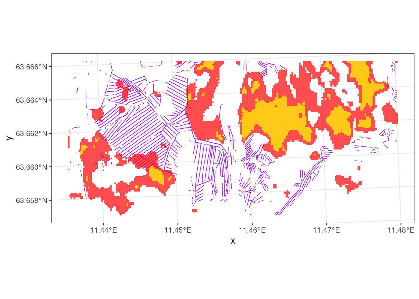
Let’s zoom in on an area just north of Tomtvatnet, and overlay the trenches data with a map of open mires (Bakkestuen et al. 2023).

bbox_new <- st_bbox(lev) # current bounding box

xrange <- bbox_new$xmax - bbox_new$xmin # range of x values
yrange <- bbox_new$ymax - bbox_new$ymin # range of y values

bbox_new[1] <- bbox_new[1] + (0.3 * xrange) # xmin - left
bbox_new[3] <- bbox_new[3] - (0.5 * xrange) # xmax - right
bbox_new[2] <- bbox_new[2] + (0.4 * yrange) # ymin - bottom
bbox_new[4] <- bbox_new[4] - (0.5 * yrange) # ymax - top

lev_crop <- lev |>
  sf::st_crop(bbox_new)

# I took the gdb file in the same folder and opened it in arcgis pro
# and exported a section of it as geoTIFF
# Raster GBD is not readable in R with GDAL <3.7
path <- "41201785_okologisk_tilstand_2022_2023/data/Myrmodell/myrmodell_levanger.tif"
mire90 <- stars::read_stars(paste0(path1, path)) |>
  st_crop(lev_bb) |> 
  setNames("prob") |>
  mutate(prob = case_when(
    prob > 900 ~ 1,
    TRUE ~ NA
  ))
stars::write_stars(mire90, "data/mire_levanger_reclassified90.tif")
saveRDS(mire90, "data/mire_levanger_reclassified90.rds")

mire70 <- stars::read_stars(path) |>
  st_crop(lev_bb) |> 
  setNames("prob") |>
  mutate(prob = case_when(
    prob > 700 ~ 1,
    TRUE ~ NA
  ))
stars::write_stars(mire70, "data/mire_levanger_reclassified70.tif")
saveRDS(mire70, "data/mire_levanger_reclassified70.rds")

mire50 <- stars::read_stars(path) |>
  st_crop(lev_bb) |> 
  setNames("prob") |>
  mutate(prob = case_when(
    prob > 500 ~ 1,
    TRUE ~ NA
  ))
stars::write_stars(mire50, "data/mire_levanger_reclassified50.tif")
saveRDS(mire50, "data/mire_levanger_reclassified50.rds")

mire10 <- stars::read_stars(path) |>
  st_crop(lev_bb) |> 
  setNames("prob") |>
  mutate(prob = case_when(
    prob > 100 ~ 1,
    TRUE ~ NA
  ))
stars::write_stars(mire10, "data/mire_levanger_reclassified10.tif")
saveRDS(mire10, "data/mire_levanger_reclassified10.rds")

#90% probability
mire90 <- readRDS("data/mire_levanger_reclassified90.rds")
mire90_crop <- mire90 |>
  st_crop(st_bbox(lev_crop))

#10% probability
mire10 <- readRDS("data/mire_levanger_reclassified10.rds")
mire10_crop <- mire10 |>
  st_crop(st_bbox(lev_crop))

ggplot() + 
  geom_sf(data = lev_crop,
          fill = "purple",
          color = "purple") +
  geom_stars(data = mire10_crop,
             downsample = 0,
             fill = "red",
             na.action = na.omit,
             alpha=.7)+
  geom_stars(data = mire90_crop,
             downsample = 0,
             fill = "yellow",
             na.action = na.omit,
             alpha=.7)+
  theme_bw()

Figure 2.2: “Zoomed in version of the previous map showing systematic trenching, but also more sporadic trenches that might be errors in the model. The red areas are open mires with 10% probability. Yellow areas are mires with 90% probability. From areal photos, the 10% probability seem to match best. Note in any case that most of the trenches are located in other nature types, mosty forests.”

The trenches model originally results in a raster with a continuous probability value for the occurrence of a trench in each 1 𝖷 1 m cell. What I show above (Figure 2.1, Figure 2.2) is a version of this data where a threshold value of 90% for the probabilities turn it into presence-absence data in the shape of polygons.

2.1 Adding AR5

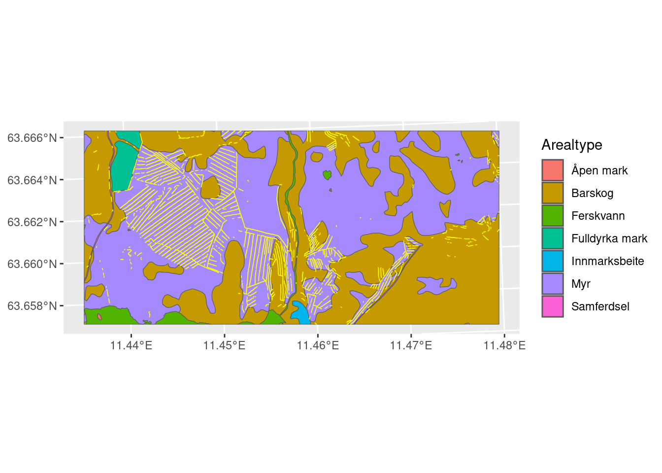
The open wetlands, shown as red areas in Figure 2.2, are largely laying outside of the systematically trenched areas. This can be because the trenched areas, which may have been open mire to begin with, now are overgrown with trees. The map of open mires is in way trained to find areas that are not trenched, so no wonder if the ecosystem condition looks good in these areas. Instead I think we should include forested mires in the Ecosystem Type (ET). We can use the mire class in the AR5 maps in addition to the open mires map. AR5 underestimates the total mire area, but it probably includes more forested mires. Another alternative would be to use the new Ecosystem Map of Norway (Strand et al. 2023), but this uses AR50, i.e. as coarser generalization of AR5.

ar5 <- readRDS("data/ar5.rds")
ggplot() + 
  geom_sf(data = ar5,
          aes(fill = Arealtype)) +
  geom_sf(data = lev_crop,
          fill = "yellow",
          color = "yellow")

Figure 2.3: “AR5 overlayed with the mire trenches data. AR5 classifies most of the systamtically trenched peatlands as mire, and some as forest.

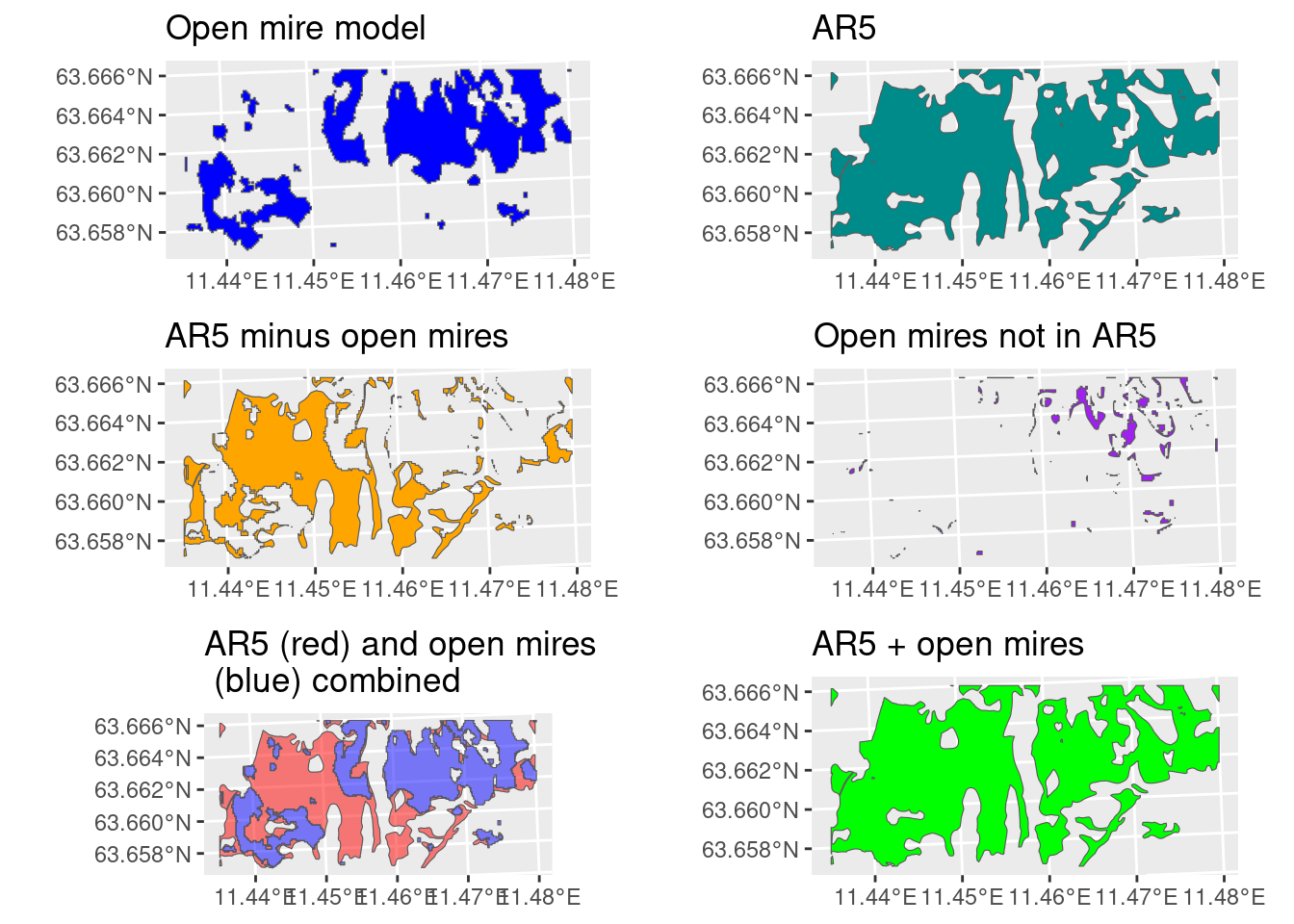
Let’s separate out the areas that are mire in AR5, but not in the open mire map, and see if adding these areas make a difference. Of coarse, we are only looking at a very small spatial extent here, and it is not representative for all the differences between AR5 and the opne mire map, but still.

# make the ecosystem delineation map into polygons
mire <- st_as_sf(mire10_crop, merge = T)
mire_gg <- ggplot(data = mire)+
  geom_sf(fill = "blue")+
  labs(title = "Open mire model")

# Filter out the mire part of AR5
ar5_myr <- ar5 |>
  filter(Arealtype == "Myr") |>
  st_cast("POLYGON")
ar5_myr_gg <- ggplot(data = ar5_myr)+
  geom_sf(fill = "cyan4")+
  labs(title = "AR5")

# Take out the open mire part of AR5 (leaving the forested peatlands)
st_erase = function(x, y) st_difference(x, st_union(st_combine(y)))
ar5_nonOpen <- ar5_myr |>
  st_erase(mire)

# Take out the AR5 part of the open mire model
only_open <- mire |>
  st_erase(ar5_myr) |>
  st_cast("MULTIPOLYGON") |>
  st_cast("POLYGON")

only_open_gg <- ggplot(data = only_open)+
  geom_sf(fill = "purple")+
  labs(title = "Open mires not in AR5")

ar5_nonOpen_gg <- 
  ggplot(data = ar5_nonOpen)+
  geom_sf(fill = "orange")+
  labs(title = "AR5 minus open mires")

# check that polygons dont overlap
check <- 
  ggplot(data = ar5_nonOpen)+
  geom_sf(fill = "red",
          alpha=.5)+
  geom_sf(data = mire,
          fill = "blue",
          alpha=.5)+
  labs(title = "AR5 (red) and open mires\n (blue) combined")

# combine into new mire map
# This first attempt with st_union produces way to many small polygon
#peatlands <- ar5_myr |>
#  st_union(mire) |>
#  st_cast("MULTIPOLYGON") |>
#  st_cast("POLYGON")

#but this works:
peatlands <- ar5_myr |>
  st_join(mire) |>
  st_intersection()

peatlands_gg <- ggplot(data = peatlands)+
  geom_sf(fill = "green")+
  labs(title = "AR5 + open mires")

ggarrange(mire_gg, 
          ar5_myr_gg, 
          ar5_nonOpen_gg, 
          only_open_gg,
          check, 
          peatlands_gg,
          ncol=2, nrow=3)

Figure 2.4: “Different combinations of the open mire model and the AR5 mire category.”

2.2 Ecosystem delineation

We presented a study area that is practically square (Figure 2.1). However, for the purpose of an ecosystem condition account or assessment, this area needs to be partitioned into unique and non-overlapping ecosystems, and our indicator needs to address the ecosystem condition the target ecosystem explicitly. The ecosystem that this indicator is aimed at is wetlands, or våtmark in Norwegian.

We might therefore need to mask our spatial data at some stage in order to exclude trenches identified in other ecosystems. However, this is problematic for several reasons.

We do not have a very precise ecosystem delineation map for wetlands, and it is not yet clear if the ecosystem should be defined as all types of wetlands, or just open wetlands. In the case of the latter, we have a quite good ecosystem map that we can use (Figure 2.2). But by excluding everything that is not open mire, we automatically exclude wetlands, or previous wetlands, that have become forested due to the lowered water table that comes from trenching. In other words, we exclude the areas that are in the worst condition. From Figure 2.2 we can see that this is a very common scenario. Alternatively, we can use things like AR5, or a combination of the two (Figure 2.4).

When it comes to updating the indicator in the future (see Chapter 4), we will be in the case that more and more trenched wetland becomes classified as other nature types, mainly forests, because that is what happens when you trench a mire. As a consequence, the indicator values will look better and better over time, reflection the land use change and the associated loss of the areas in worst condition. This is a well known issue in ecosystem accounting (ref Jacobson).

We recommend for this indicator to delineate the nature type as open mires in the open mire model (Bakkestuen et al. 2023), in combination with mires in AR5 (Figure 2.4; last pane).

References

Bakkestuen, V., Venter, Z., Ganerød, A.J., and Framstad, E. 2023. Delineation of Wetland Areas in South Norway from Sentinel-2 Imagery and LiDAR Using TensorFlow, U-Net, and Google Earth Engine. Remote Sensing 15(5): 1203. doi:10.3390/rs15051203.

Jansson, U., Bakkestuen, V., Lyngstad, A., and Mienna, I.M. 2024. Utvikling av grøftekart i myr og torvmark i norge med hjelp av dyplæring.

Strand, G.-H., Framstad, E., and Opsahl, L.A. 2023. Hovedøkosystemkart for norge. NIBIO Rapport.