7 Freshwater ecosystem

The Nature Index (NI) is calculated as a weighted mean of a range of different indicators. Each indicator is first scaled with respect to its reference value such that it takes on values between 0 and 1, where 0 corresponds to a species (group)/habitat type being extinct/completely lost, and 1 corresponds to an abundance of a species /group)/habitat type as we would expect it in an ecosystem with as little as possible human disturbance. In the case of semi-natural ecosystems, value 1 represents the indicator state in a well-managed ecosystem. After scaling, each indicator is assigned a composite weight that is dependent on trophic group, relative area for which data are available, and key indicator status. In early versions of NI, ecosystem fidelity (given as % of the indicator distributed across different ecosystems) was also used for assigning weights; however, as of NI2020, this is no longer done as there is no reason to down-weigh an indicator in ecosystem A just because it also appears in ecosystem B. NI for a given ecosystem is the calculated as a weighted average of all relevant indicators. For more information on the Nature Index framework, please refer to the sources provided in Chapter XX: “Links and references”.

In the following, I describe the workflow for calculating NI2025 for freshwater ecosystems.

The workflow is largely based on scripts developed for automating NI calculations for ecosystem condition accounts and collated in the “NIflex” package (https://github.com/NINAnor/NIflex). Most operations have previously been coded in the “NIcalc” package (https://github.com/NINAnor/NIcalc). The workflow here contains the following steps:

• Retrieval of necessary data from NI database
• Calculation of NI2025
• Visualization of NI2025 as time-series plots (traditional and using density ridges) and maps
• Local storage of results
• Remote storage of results in NI database to be used for visualizations on the webpage

A note on reference value uncertainty

Reference values can be – and have been – entered into the NI database either with or without associated uncertainty. Most reference values have been set early on in the NI work (period 2010-2014) and not changed since; a few have been updated or re-calibrated since. The approaches for setting reference values across the indicator set have been extremely variable, and neither particularly structured nor harmonized. This is one of the reasons why reference value uncertainty has not been included in previous iterations of NI (NI2010, NI2015, NI2020).

Investigating the effects of including reference value uncertainty on NI calculations is not part of the commission for NI2025, either. As such, also NI2025 is calculating without accounting for reference value uncertainty.

This should, however, be considered for future work, ideally in combination with a re-assessment and structured and standardized update of reference values across the indicator set. Fortunately, the option for using uncertain reference values in practice is already coded into “NIcalc”; specifically, within NIcalc::calculate_Index() there is a function called setCalculationParameters(), and the argument stochastic of that function has to be changed from “obervations” to “both” to include uncertainty in both yearly indicator values and reference values.

7.1 General setup

There are a few variables that are used to control execution of parts of the code in this chapter. We start off by defining these here:

## Years
years <- c("2000", "2010", "2014", "2019", "2024")

## Year for map plots
mapYear <- max(years)

## Missing value imputation
NAImputation <- TRUE

## Key indicator weighing
KeyIndicators <- TRUE
KeyWeight <- 0.5

## Area weighing
AreaWeights <- TRUE # Yes

## Trophic weighing
TrophicWeights <- TRUE # Yes

## Norwegian indicator names
norwegianNames <- TRUE

## Output type
OutputType <- "NatureIndex"

## Nature Index ecosystem 
#Ecosystem <- c("Forest", "Skog")
#Ecosystem <- c("Mountain", "Fjell")
#Ecosystem <- c("Wetlands", "Våtmark")
#Ecosystem <- c("OpenLowland", "Åpent lavland")
Ecosystem <- c("Freshwater", "Ferskvann")
#Ecosystem <- c("Coast", "Kystvann")
#Ecosystem <- c("Ocean", "Hav")

EC_ecosystem <- NULL
ecosystem_use <- Ecosystem[2]

## Thematic index name
theme <- "None"

## Options for dropping indicators
DropIndMode <- "pre-defined"
DropIndList <- NULL

## Diagnostics imputation
Diagnostics <- TRUE # Yes

## Test run (10 vs. 1000 iterations in simulation)
#TestRun <- TRUE # Yes
TestRun <- FALSE # No

## Shapefiles library path
shapeLibraryPath <- Sys.getenv("NI_shapeLibraryPath", unset = "data/Shapefiles")
#shapeLibraryPath <- "P:/412430_naturindeks/Beregninger/Shapefiles" # for running locally on NINA PC
#shapeLibraryPath <- "/data/P-Prosjekter2/412430_naturindeks/Beregninger/Shapefiles" # for running on NINA RStudio server

Additionally, we will define and set a seed to ensure reproducibility of the simulations:

mySeed <- 0
set.seed(mySeed)

Since calculations are quite time-consuming, I will also code in a switch to control when they are to be re-run. As a default, R will check if any files with names corresponding to the saved results are already present in the working directory and only re-run calculations if that is not the case. If the switch forceRerun is set to TRUE, calculations will be re-run irrespective of files present.

forceReRun <- FALSE

7.2 Connect to the Nature Index Database

To access and download indicator data, we need to retrieve a token from the NI database. For that to work, we need access to our NI database access credentials; we retrieve those from environmental variables (if you have not saved them as environmental variables, you can find the code for doing that in chapter 0; alternatively, you can also manually set them here):

NIdb_username <- Sys.getenv("NIdb_username")
NIdb_password <- Sys.getenv("NIdb_password")

7.3 Retrieve data and calculate NI2025

The entire workflow for NI calculations is contained in NIflex::calclulateCustomNI() and contains the following steps:

1. Data download via NIcalc::importDatasetApi
2. Assembly of input data for calculations via NIcalc::assembleNiObject
3. Optional: run dataset diagnostics via NIcalc::imputeDiagnostics
4. Optional: impute missing data via NIcalc::imputeData (which uses mice::mice)
5. Index calculation via NIcalc::calculateIndex

The list of indicators that is used to calculate NI for specific ecosystems is retrieved directly from the NI database and is shown further down (after calculations). NIflex does provide the option to drop selected indicators; however, as the NI database is currently updated in terms of active/inactive indicators for NI2025, we do not need to drop any additional indicators.

if(!file.exists(paste0("data/NI2025_Data_", Ecosystem[1], ".rds")) | forceReRun){
  
  ## Assign indicator set
  indicators_use <- NULL
  
  ## Make list of indicators to drop
  dropInd <- selectDropIndicators(DropIndMode = DropIndMode,
                                  OutputType = OutputType,
                                  ecosystem = ifelse(OutputType %in% c("NatureIndex", "EcologicalCondition"), ecosystem_use, NULL),
                                  customList = DropIndList)
  
  ## Calculate index for specified ecosystem/indicators
  CustomNI <- calculateCustomNI(ecosystem = ecosystem_use,
                                indicators = indicators_use,
                                theme = theme,
                                dropInd = dropInd,
                                username = NIdb_username,
                                password = NIdb_password,
                                KeyIndicators = KeyIndicators,
                                KeyWeight = KeyWeight,
                                AreaWeights = AreaWeights,
                                TrophicWeights = TrophicWeights,
                                NAImputation = NAImputation,
                                years = years,
                                OutputType = OutputType,
                                funArguments = funArguments,
                                Diagnostics = Diagnostics,
                                TestRun = TestRun,
                                norwegianNames = norwegianNames,
                                saveSteps = TRUE)
}

7.4 Storing numerical results locally

NIflex::calculateCustomIndex() automatically saves the results into the working directory as “CustomIndex_Data.rds”. Since we are now handling multiple indices (NI for all seven ecosystems, as well as a couple of thematic indices), we want to make sure they all have logical and individual file names. We therefore rename the output file:

if(!file.exists(paste0("data/NI2025_Data_", Ecosystem[1], ".rds")) | forceReRun){
  
  file.rename(from = "CustomIndex_Data.rds",
              to = paste0("data/NI2025_Data_", Ecosystem[1], ".rds"))
}

The output file contains a lot of information and metadata on the indicator set, calculated index, spatial units, calculation parameters, etc. It’s also an R object, making it not the best “reference” for looking up values for non-specialists (including the “Faggruppe” for NI that will be responsible for interpreting and reporting results). For that reason, we will summarise the most important numbers and save them as .csv files in designated folders. For now, we will do this for the following parts of the results:

• Indicator list (incl. metadata)
• Indicator weights
• Statistical summary of calculated index distributions

if(!exists("CustomNI")){
  CustomNI <- readRDS(paste0("data/NI2025_Data_", Ecosystem[1], ".rds"))
}

## Make target folder (if non-existent)
saveFolder <- paste0("results_", Ecosystem[1])
if(!dir.exists(saveFolder)){
  dir.create(saveFolder)
}

## Save indicator list
indicatorList <- CustomNI$CustomIndex$wholeArea$`2024`$indicatorData %>%
  dplyr::select(id, name, keyElement, functionalGroup, scalingModel)

readr::write_excel_csv(indicatorList, file = paste0(saveFolder, "/indicatorList.csv"))

## Save summarised indicator weights
indicatorWeights <- data.frame(
  name = rownames(NIcalc::summaryWeights(CustomNI$CustomIndex$wholeArea)),
  weight = NIcalc::summaryWeights(CustomNI$CustomIndex$wholeArea)[,2],
  row.names = NULL) %>%
  dplyr::mutate(weigth_percent = round(weight*100, digits = 2))

readr::write_excel_csv(indicatorWeights, file = paste0(saveFolder, "/indicatorWeights.csv"))

## Make and save statistical summary of calculated index distributions
indexSummary <- data.frame()

for(a in 1:length(CustomNI$CustomIndex)){
  for(t in 1:length(years)){
    
    indexSum_a_t <- data.frame(
      Area = names(CustomNI$CustomIndex)[a],
      Year = years[t],
      value = CustomNI$CustomIndex[[a]][[t]]$index) %>%
      dplyr::group_by(Area, Year) %>%
      dplyr::summarise(mean = mean(value),
                       median = median(value),
                       sd = sd(value),
                       rel_sd = sd/mean,
                       q025 = quantile(value, probs = 0.025),
                       q05 = quantile(value, probs = 0.05),
                       q25 = quantile(value, probs = 0.25),
                       q75 = quantile(value, probs = 0.75),
                       q95 = quantile(value, probs = 0.95),
                       q975 = quantile(value, probs = 0.975),
                       .groups = "keep") %>%
      dplyr::ungroup()
    
    indexSum_a_t[, 3:12] <- round(indexSum_a_t[, 3:12], digits = 3)
    
    indexSummary <- indexSummary %>%
      dplyr::bind_rows(indexSum_a_t)
  }
}

indexSummary <- indexSummary %>%
  dplyr::mutate(Area = dplyr::case_when(Area == "wholeArea" ~ "All Norway",
                                        Area == "E" ~ "Eastern Norway",
                                        Area == "S" ~ "Southern Norway",
                                        Area == "W" ~ "Western Norway",
                                        Area == "N" ~ "Northern Norway",
                                        Area == "C" ~ "Central Norway",
                                        TRUE ~ Area))

readr::write_excel_csv(indexSummary, file = paste0(saveFolder, "/indexStatSummary.csv"))

Note that all steps related to summarising and saving numerical data are only required if we have just re-run calculations.

Some numerical results also have to be sent back to the NI database. This is done in the last part of this script (see below).

7.5 Overview over indicator set and weights

This and the following chapter present the calculated NI2025 for the ecosystem Freshwater. Irrespective of whether we have just re-run calculations, we start by loading in the complete results file, as well as summary tables created in the previous section:

saveFolder <- paste0("results_", Ecosystem[1])

Index <- readRDS(paste0("data/NI2025_Data_", Ecosystem[1], ".rds"))$CustomIndex

indicatorList <- readr::read_csv(paste0(saveFolder, "/indicatorList.csv"))
indicatorWeights <- readr::read_csv(paste0(saveFolder, "/indicatorWeights.csv"))
indexSummary <- readr::read_csv(paste0(saveFolder, "/indexStatSummary.csv"))

The following table lists all indicators that are part of NI2025 for Freshwater (Ferskvann). More information on each indicator can be found in the NI database (https://naturindeks.nina.no/). Visualizations of indicator values and trends are shown in Chapter 1.

Table 7.1: List of indicators included in NI2025 for ecosystem Freshwater. id and name are consistent with use in the NI database. Indicators with keyElement = TRUE are treated as key indicators (nøkkelindikatorer) and assigned extra weight. Functional group also affects the weight attributed to indicators. Scaling model = Low means that indicator values > reference are considered good, while scaling model Max assumes that the reference is a maximum threshold, and values exceeding it are bad.

id	name	keyElement	functionalGroup	scalingModel
3	Alge på bjørk	FALSE	Primærprodusent	Low
5	Alm	FALSE	Primærprodusent	Low
9	Bananslørsopp	FALSE	Primærprodusent	Low
10	Begerfingersopp	FALSE	Nedbryter	Low
399	Bjørkefink	FALSE	Mellompredator	Low
23	Blåbær	TRUE	Primærprodusent	Low
398	Bokfink	FALSE	Mellompredator	Low
29	Brunbjørn	FALSE	Topp-predator	Low
351	Dagsommerfugler i skog	FALSE	Plantespisere og filterspisere	Low
410	Dompap	FALSE	Mellompredator	Low
314	Duetrost	FALSE	Mellompredator	Low
41	Eldre lauvsuksesjon (MiS)	TRUE	Ikke egnet	Low
42	Elg	FALSE	Plantespisere og filterspisere	Low
49	Fiolgubbe	FALSE	Primærprodusent	Low
286	Fjellvåk	FALSE	Topp-predator	Low
392	Flaggspett	FALSE	Mellompredator	Low
28	Flekkhvitkjuke	FALSE	Nedbryter	Low
110	Fossenever	FALSE	Primærprodusent	Low
407	Fuglekonge	FALSE	Mellompredator	Low
60	Gamle trær (MiS)	TRUE	Ikke egnet	Low
434	Gammel skog	TRUE	Ikke egnet	Low
62	Gaupe	FALSE	Topp-predator	Low
408	Gjerdesmett	FALSE	Mellompredator	Low
414	Grå fluesnapper	FALSE	Mellompredator	Low
317	Granmeis	FALSE	Mellompredator	Low
318	Gransanger	FALSE	Mellompredator	Low
69	Grønn fåresopp	FALSE	Primærprodusent	Low
394	Grønnspett	FALSE	Mellompredator	Low
335	Gulsanger	FALSE	Mellompredator	Low
412	Hagesanger	FALSE	Mellompredator	Low
77	Hjort	FALSE	Plantespisere og filterspisere	Low
319	Hønsehauk	FALSE	Topp-predator	Low
359	Humler i skog	FALSE	Plantespisere og filterspisere	Low
86	Isterviersumpskog	FALSE	Primærprodusent	Low
400	Jernspurv	FALSE	Mellompredator	Low
88	Jerv	FALSE	Topp-predator	Low
89	Jordstjerner	FALSE	Nedbryter	Low
322	Kongeørn	FALSE	Topp-predator	Low
98	Kopperrød slørsopp	FALSE	Primærprodusent	Low
100	Kusymre	FALSE	Primærprodusent	Low
106	Lappkjuke	FALSE	Nedbryter	Low
419	Liggende død ved – mengde	TRUE	Nedbryter	Low
108	Liggende død ved (MiS) – arealandel	FALSE	Nedbryter	Low
109	Lirype	FALSE	Plantespisere og filterspisere	Low
324	Løvsanger	FALSE	Mellompredator	Low
325	Måltrost	FALSE	Mellompredator	Low
326	Munk	FALSE	Mellompredator	Low
396	Nøtteskrike	FALSE	Mellompredator	Low
130	Olavsstake	FALSE	Primærprodusent	Low
384	Orrfugl	FALSE	Plantespisere og filterspisere	Low
153	Rådyr	FALSE	Plantespisere og filterspisere	Low
409	Ringdue	FALSE	Mellompredator	Low
406	Rødstjert	FALSE	Mellompredator	Low
402	Rødstrupe	FALSE	Mellompredator	Low
395	Rødvingetrost	FALSE	Mellompredator	Low
433	Rogn-Osp-Selje	TRUE	Primærprodusent	Low
332	Smågnagere - skogbestander	TRUE	Plantespisere og filterspisere	Low
418	Stående død ved – mengde	TRUE	Nedbryter	Low
183	Stående død ved (MiS) – arealandel	FALSE	Nedbryter	Low
186	Storfugl	FALSE	Plantespisere og filterspisere	Low
187	Storpiggslekten (sopp)	FALSE	Primærprodusent	Low
328	Svarthvit fluesnapper	FALSE	Mellompredator	Low
403	Svartmeis	FALSE	Mellompredator	Low
194	Svartnende kantarell	FALSE	Primærprodusent	Low
195	Svartsonekjuke	FALSE	Nedbryter	Low
393	Svartspett	FALSE	Mellompredator	Low
397	Svarttrost	FALSE	Mellompredator	Low
436	Tamrein	FALSE	Plantespisere og filterspisere	Low
330	Toppmeis	FALSE	Mellompredator	Low
207	Trær med hengelav (MiS)	FALSE	Primærprodusent	Low
405	Trekryper	FALSE	Mellompredator	Low
401	Trepiplerke	FALSE	Mellompredator	Low
209	Ulv	FALSE	Topp-predator	Low

Indicators are assigned weights (= contributions to NI) based on their functional group (trophic weight), the relative extent of area for which data is available (area weight), and whether or not they are considered key indicators (all key indicators together are given 50% of the total weight in NI calculations).

For NI2025, the top 35 indicator weights for ecosystem Freshwater are attributed as shown below. Note that blue bars represent the key indicators, while grey bars are “normal” (= non-key) indicators.

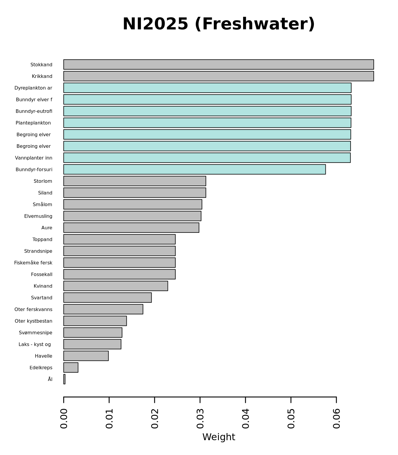
This figure, as well as an extended version showing weights for all included indicators, can be found in the ecosystem-specific results folder under “Plots”.

A table containing all indicator weights in numerical format is saved under results_Freshwater/indicatorWeights.csv.

7.6 Visualizing results

Traditionally, NI has been presented using two different types of visualizations: time-series graphs of medians with 95% confidence intervals and maps of median values (for each year).

The graphical presentation of NI2025 has been extended and will include the following:

• Time-series graphs of medians and 95% confidence intervals, for the area-aggregated mean as before but also including values for each of the five major regions of Norway

• Time-series graphs of complete values distributions for the area-aggregated means and for each of the five major regions of Norway

• Maps of median values, uncertainty (represented as interquartile distance), and statistical location displacement

Below we present each one of these. In addition to the displays in this document, all plots are also saved as .pdf and .svg files in the “Plots” subfolder in the respective ecosystem’s results folder (results_Freshwater).

Dynamic versions of median/95% CI time series and median/uncertainty maps will be included on the new webpage for NI2025 (under development).

7.6.1 Time-series of medians and 95% CIs

For just getting a quick look at the NI values for all of Norway over time, we can use the original plotting function from the “NIcalc” package:

plot(Index$wholeArea, main = paste0("NI2025 ", Ecosystem[1]), cex = 1, lwd = 2, shade = TRUE)

NIflex::plotNI_StandardTS() gives us an extended version of this type of plot which also includes values for each major region of Norway separately:

standardTS1 <- NIflex::plotNI_StandardTS(Index = Index,
                                         plotTitle = Ecosystem[1],
                                         addAverage = TRUE,
                                         truncateY = FALSE)
standardTS1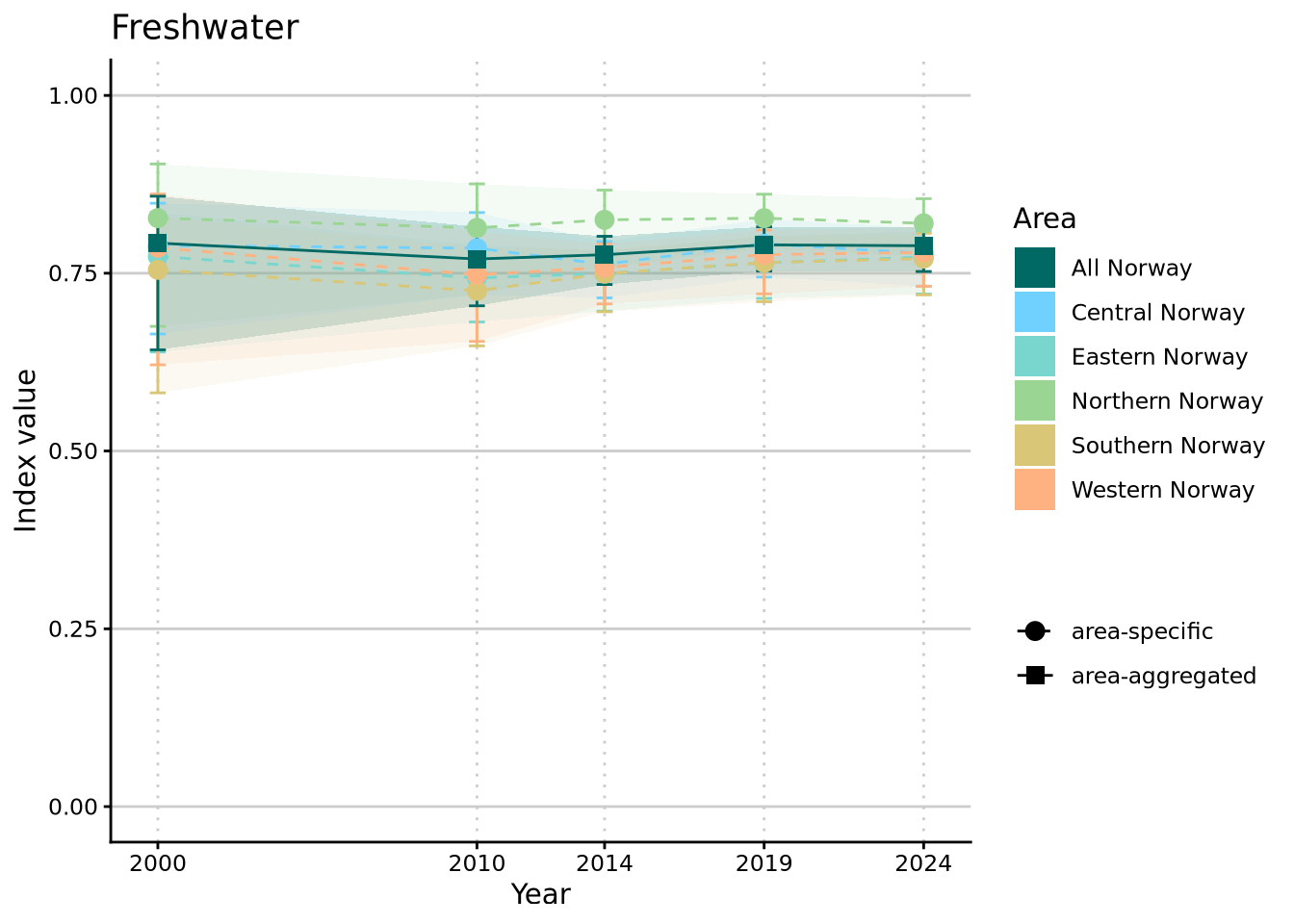

The plot above shows the development of NI over time on the complete scale of values from 0 to 1. This gives a good idea of where values lie relative to the ideal of “good condition” / “as little as possible human impacted ecosystem” but is not necessarily the best for looking at between-year changes in NI. The latter is more obvious with a truncated y axis that is limited to the range of values that this NI actually takes:

standardTS2  <- NIflex::plotNI_StandardTS(Index = Index,
                                          plotTitle = Ecosystem[1],
                                          addAverage = TRUE,
                                          truncateY = TRUE)
standardTS2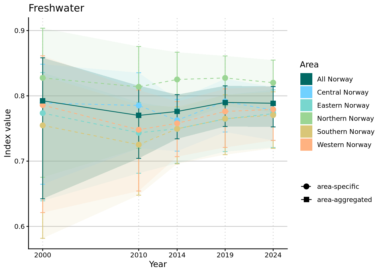

7.6.2 Time-series of entire uncertainty distributions

NI is calculated through simulation and bootstrap; as such, the results consist of 1000 replicate values. The distribution of these values does not necessarily have to be normal and it is good to have a look at what the entire value distributions look like, not just their medians and quantiles/confidence intervals. That’s what NIflex::plotNI_DensityRidgeTS() is for. When plotting for the area-aggregated estimates (entire Norway), we get:

densTS1 <- NIflex::plotNI_DensityRidgeTS(Index = Index, 
                                         OutputType = OutputType, 
                                         ecosystem = ecosystem_use, 
                                         theme = theme,
                                         allAreas = FALSE, 
                                         selectedArea  = "wholeArea")
densTS1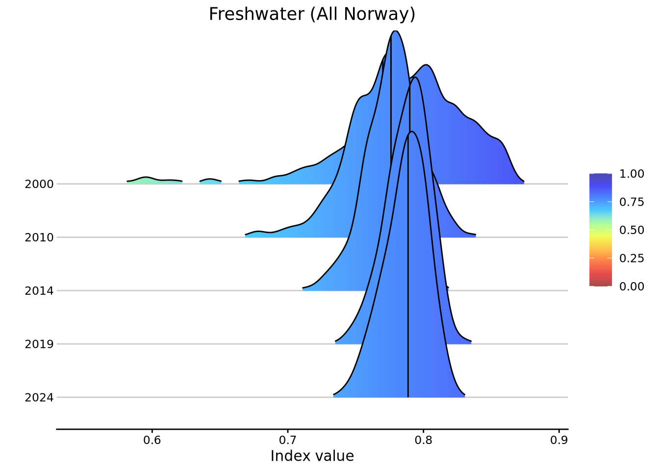

And the same separated by area:

densTS2 <- NIflex::plotNI_DensityRidgeTS(Index = Index, 
                                         OutputType = OutputType, 
                                         ecosystem = ecosystem_use, 
                                         theme = theme,
                                         allAreas = TRUE)
densTS2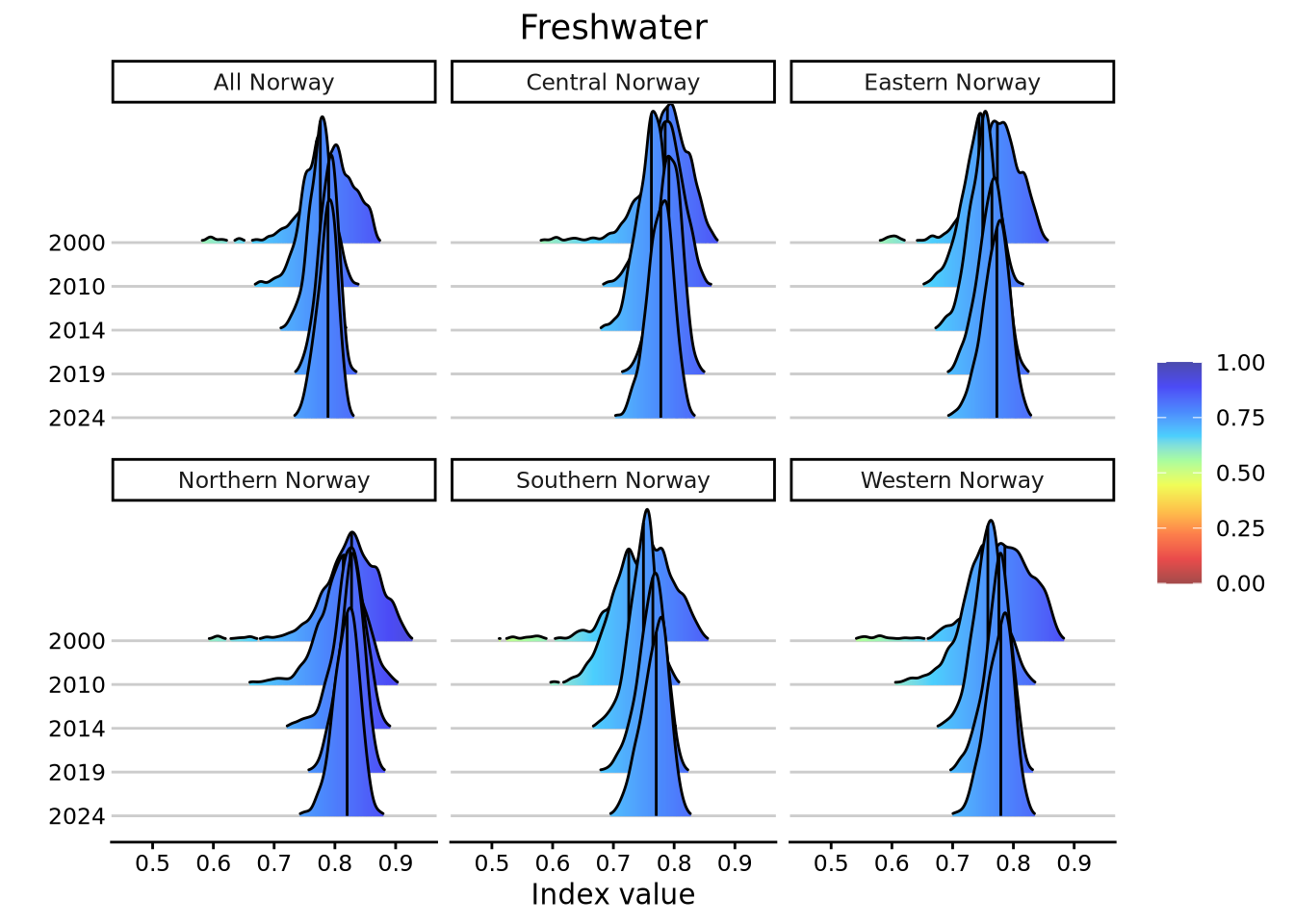

7.6.3 Median, uncertainty, and displacement maps

Maps are very popular tools for disseminating results nowadays, but their major drawback is that usually, they are presented without associated uncertainty. For that reason, NI2025 will have an added focus on visualizing uncertainty associated with maps, too. There are two key elements of uncertainty in NI calculations:

1. Uncertainty characterizing the distribution of predicted NI values. This is the same type of uncertainty we also visualized in time series above and it is a quantitative measure of the spread of the predicted index values. In the map plots, we use the confidence interval width (97.5% quantile - 2.5% quantile) for visualizing uncertainty, but other measures (e.g. standard deviation, relative standard deviation, additional quantiles) can be found in the statistical summary table results_Freshwater/indexStatSummary.csv.

2. Statistical location displacement. This is a measure that quantifies the degree to which the median of index calculations is “displaced” during the aggregation process. This displacement is a statistical artifact resulting from truncation of indicator values that exceed their reference value. It has always been a property of the NI’s statistical framework and is not considered a major issue. However, it is important to keep location displacement in mind when interpreting results, i.e. median values with a large associated displacement should be interpreted with extra caution.

Before proceeding, we first need to combine our index values with corresponding geospatial data. The latter is contained in shapefiles archived on NINA’s internatal data systems under “P:/412430_naturindeks/Beregninger/Shapefiles”. The shapefiles are derived from spatial data stored in the NI database; if you are in need of access to these shapefiles, please contact the NI core team at NINA (naturindeks@nina.no) or the database administrator (siw.berge@nina.no).

CustomNI_map <- NIflex::geomapNI(Index = Index, 
                                 year = mapYear, 
                                 OutputType = OutputType, 
                                 ecosystem = ecosystem_use,
                                 shapeLibraryPath = shapeLibraryPath)

Then we are ready to plot the pair of maps representing the median values and value uncertainty:

NIflex::plotNI_Map(shp = CustomNI_map, 
                   year = mapYear, 
                   OutputType = OutputType, 
                   ecosystem = ecosystem_use,
                   plotMedian = TRUE, plotCI = TRUE, plotDisplacement = FALSE, 
                   interactiveMap = TRUE)

And we can do the same with location displacement instead of CI width:

NIflex::plotNI_Map(shp = CustomNI_map, 
                   year = mapYear, 
                   OutputType = OutputType, 
                   ecosystem = ecosystem_use,
                   plotMedian = TRUE, plotCI = FALSE, plotDisplacement = TRUE, 
                   interactiveMap = TRUE)

Static versions of all types of maps for the different years are saved under results_Freshwater/Plots/Maps. The code for generating them is below:

## Make directory
if(!dir.exists(paste0(plotPath, "/Maps"))){
  dir.create(paste0(plotPath, "/Maps"))
}


for(t in 1:length(years)){
  
  ## Set up map base
  CustomNI_map <- NIflex::geomapNI(Index = Index, 
                                 year = years[t], 
                                 OutputType = OutputType, 
                                 ecosystem = ecosystem_use,
                                 shapeLibraryPath = shapeLibraryPath)
  
  ## Draw maps
  mapMedian <- NIflex::plotNI_Map(shp = CustomNI_map, 
                                  year = years[t], 
                                  OutputType = OutputType, 
                                  ecosystem = ecosystem_use,
                                  plotMedian = TRUE, plotCI = FALSE, plotDisplacement = FALSE, 
                                  interactiveMap = FALSE)
  mapCI <- NIflex::plotNI_Map(shp = CustomNI_map, 
                              year = years[t], 
                              OutputType = OutputType, 
                              ecosystem = ecosystem_use,
                              plotMedian = FALSE, plotCI = TRUE, plotDisplacement = FALSE, 
                              interactiveMap = FALSE)
  mapDisp <- NIflex::plotNI_Map(shp = CustomNI_map, 
                                year = years[t], 
                                OutputType = OutputType, 
                                ecosystem = ecosystem_use,
                                plotMedian = FALSE, plotCI = FALSE, plotDisplacement = TRUE, 
                                interactiveMap = FALSE)
  
  ## Save as multipage pdf
  pdf(paste0(plotPath, "/Maps/NI2025_", Ecosystem[1], "_", years[t], ".pdf"), width = 5, height = 5)
  
  print(mapMedian)
  print(mapCI)
  print(mapDisp)
  
  dev.off()
  
  ## Save as svg
  svglite(paste0(plotPath, "/Maps/NI2025_", Ecosystem[1], "_Median_", years[t], ".svg"), width = 5, height = 5)
  print(mapMedian)
  dev.off()
  
  svglite(paste0(plotPath, "/Maps/NI2025_", Ecosystem[1], "_CIwidth_", years[t], ".svg"), width = 5, height = 5)
  print(mapCI)
  dev.off()
  
  svglite(paste0(plotPath, "/Maps/NI2025_", Ecosystem[1], "_Displacement_", years[t], ".svg"), width = 5, height = 5)
  print(mapDisp)
  dev.off()
  
  
}

7.7 Addendum: thematic indices

As of NI2025, all previously published thematic indices have been discontinued. We have, however, had a request to provide the thematic indices for “Forsuring ferskvann” (= freshwater acidification) and “Eutrofiering ferskvann” (= freshwater eutrophication) as tools to aid with interpretation of NI for freshwater ecosystems.

Routines for calculating thematic indices have been streamlined within “NIflex”, and we’ll refer to package documentation for details on the implementation.

Below, we calculate and then visualize the two requested thematic indices.

7.7.1 Freshwater acidification

The following table shows the indicators that are part of the thematic index for freshwater acidification:

Table 7.2: List of indicators included in thematic index for freshwater acidification. id and name are consistent with use in the NI database. Key indicator (nøkkelindikator) weights are not used for calculating thematic indices. Functional group also affects the weight attributed to indicators. Scaling model = Low means that indicator values > reference are considered good, while scaling model Max assumes that the reference is a maximum threshold, and values exceeding it are bad.

id	name	functionalGroup	scalingModel
231	Bunndyr-forsuringsindeks (Raddum 1)	Mellompredator generalist	Low
36	Dyreplankton artssammensetning	Plantespisere og filterspisere	Low
233	Begroing elver forsurings indeks	Primærprodusent generalist	Low
50	Aure	Topp-predator generalist	Low

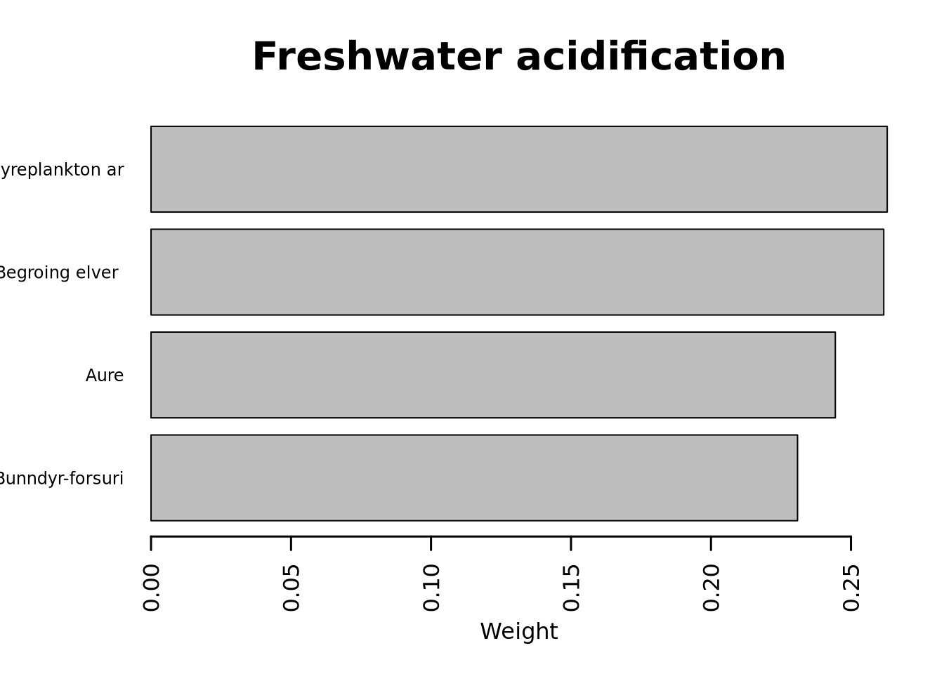
The indicator weights are shown below.

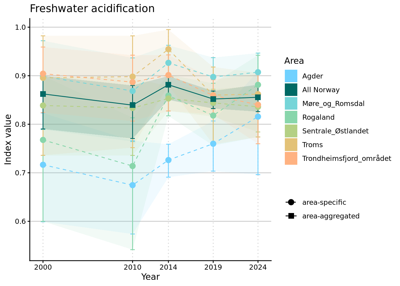
The thematic index has developed over time as follows:

The complete indicator distributions are visualized next:

7.7.2 Freshwater eutrophication

The following table shows the indicators that are part of the thematic index for freshwater eutrophication:

Table 7.3: List of indicators included in thematic index for freshwater eutrophication. id and name are consistent with use in the NI database. Key indicator (nøkkelindikator) weights are not used for calculating thematic indices. Functional group also affects the weight attributed to indicators. Scaling model = Low means that indicator values > reference are considered good, while scaling model Max assumes that the reference is a maximum threshold, and values exceeding it are bad.

id	name	functionalGroup	scalingModel
228	Bunndyr-eutrofieringsindeks (ASPT)	Mellompredator generalist	Low
11	Begroing elver eutrofierings indeks	Primærprodusent generalist	Low
146	Planteplankton innsjøer	Primærprodusent generalist	Low
213	Vannplanter innsjø	Primærprodusent generalist	Low

The indicator weights are shown below.

The thematic index has developed over time as follows:

The complete indicator distributions are visualized next: