23 Climate indicators explained
Author and date:
Anders L. Kolstad
March 2023
| Ecosystem | Økologisk.egenskap | ECT.class |
|---|---|---|
| All | Abiotiske egenskaper | Physical state characteristics |
23.1 Introduction
This chapters describes the development of a workflow for generating or preparing indicators based on interpolated climate data from SeNorge. I describe the process using dummy data and also discuss alternate approaches and dead ends that occured in the development process. For a succinct workflow example for a specific indicator, see Median summer temperature.
23.2 About the underlying data
The data is in a raster format and extends back to 1957 in the form of multiple interpolated climate variables. The spatial resolution is 1 x 1 km.
23.2.1 Representativity in time and space
The data includes the last normal period (1961-1990) which defines the reference condition for climate variables. Therefore the temporal resolution is very good. Also considering the daily resolution of the data.
Spatially, a 1x1 km resolution is sufficient for most climate variables, esp. in homogeneous terrain, but this needs to be evaluation for each variable and scenario specifically.
23.4 Collinearities with other indicators
Climate variables are most likely to be correlated with each other (e.g. temperature and snow). Also, some climate variables are better classed as pressure indicators, and these might have a causal association with several condition indicators.
23.5 Reference condition and values
23.5.1 Reference condition
The reference condition for climate variables is defined as the normal period 1961-1990.
23.5.2 Reference values, thresholds for defining good ecological condition, minimum and/or maximum values
Un-scaled indicator value = median value over 5 year periods (5 years being a pragmatic choice. It is long enough to smooth out a lot of inter-annual variation, and it’s long enough to enable estimating errors)
Upper reference level (best possible condition) = median value from the reference period
Thresholds for good ecosystem condition = 2 standard deviation units away from the upper reference level for the climate variable during the reference period.
Lower reference values (two-directional) = 5 standard deviation units for the climate variable during the reference period (implies linear scaling).
The choice to use 2 SD units as the threshold values is a subjective choice in many ways, and not founded in any empirical or known relationship between the indicators and ecosystem integrity. The value comes from the common practice of calling something extreme weather when it is outside 2 SD units of the current running average. So, if the indicator value today is <0.6 it implies that the mean for that variable over the last year would have been referred to as extreme if it had occurred between 1961 and 1990. This is I think a conservative threshold, since one would/could call it extreme if only one year is outside the 2SD range, and having the mean of 5 years being outside this range is really extreme.
23.6 Uncertainties
For the indicator map (1 x 1 km raster) there is no uncertainty associated with the indicator values. For aggregated indicator values (e.g. for regions), the uncertainty in the indicator value is calculated from the spatial variation in the indicator values via bootstrapping. This might, however, be changed later to the temporal variation between the five years of each period.
23.7 References
rr and tm are being download from: https://thredds.met.no/thredds/catalog/senorge/seNorge_2018/Archive/catalog.html
23.8 Analyses
23.8.1 Data set
The data is downloaded to a local NINA server, and updated regularly.
path <- ifelse(dir == "C:",
      "R:/GeoSpatialData/Meteorology/Norway_SeNorge2018_v22.09/Original",
      "/data/R/GeoSpatialData/Meteorology/Norway_SeNorge2018_v22.09/Original")
This folder contains folder for the different parameters
(files <- list.files(path))
#>  [1] "age"        "fsw"        "gwb_eva"    "gwb_gwtcl"
#>  [5] "gwb_q"      "gwb_sssdev" "gwb_sssrel" "lwc"
#>  [9] "qsw"        "rr_tm"      "sd"         "sdfsw"
#> [13] "swe"
This table explains them in more detail
senorgelayers <- read_delim("data/senorgelayers.txt",
    delim = "\t", escape_double = FALSE,
    trim_ws = TRUE)
DT::datatable(senorgelayers)
Figure 18.1: Table explaining the available climate parameters in the data set.
Here is the content of one of these folders (first 10 entries)
(files_tm <- list.files(paste0(path, "/rr_tm")))[1:10]
#>  [1] "seNorge2018_1957.nc" "seNorge2018_1958.nc"
#>  [3] "seNorge2018_1959.nc" "seNorge2018_1960.nc"
#>  [5] "seNorge2018_1961.nc" "seNorge2018_1962.nc"
#>  [7] "seNorge2018_1963.nc" "seNorge2018_1964.nc"
#>  [9] "seNorge2018_1965.nc" "seNorge2018_1966.nc"
There are 67 files, i.e. 67 years of data, one file per year.
Importing (proxy) file:
tg_1957 <- stars::read_ncdf(paste0(path, "/rr_tm/seNorge2018_1957.nc"),
                            var="tg")
#> Large netcdf source found, returning proxy object.
I know the CRS, so setting it manually. Although I cannot rule out 32633, I don’t think it matters.
st_crs(tg_1957) <- 25833The data has three dimension
dim(tg_1957)
#>    X    Y time
#> 1195 1550  365
Initially the data had four attributes, but I subsettet to only include tg.
names(tg_1957)
#> [1] "tg"
tg_1957 is a stars proxy object and most commands will not initiate any change until later, typically I write to file and all the lazy operations are done in squeal. Therefore, I will prepare a test data set, which is smaller and which I can import to memory. Then I can perform the operations on that data set and we can see the results.
23.8.1.1 Dummy data
This test data is included in the {stars} package
tif = system.file("tif/L7_ETMs.tif", package = "stars")
t1 = as.Date("1970-05-31")
x = read_stars(c(tif, tif, tif, tif), along =
                  list(time = c(t1, t1+1, t1+50, t1+100)),
               RasterIO = list(nXOff = c(1),
                               nYOff = c(1),
                               nXSize = 50,
                               nYSize = 50,
                               bands = c(1:6)))
A single attribute
names(x)
#> [1] "L7_ETMs.tif"
I can rename it like this
x <- setNames(x, "Attribute_A")And I can add another dummy attribute.
The dummy data also has four dimensions
dim(x)
#>    x    y band time
#>   50   50    6    4
X and y area the coordinates. Band is an integer:
st_get_dimension_values(x, "band")
#> [1] 1 2 3 4 5 6
I will remove the band dimension.
Time is four dates covering four months in 1970:
(oldTime <- st_get_dimension_values(x, "time"))
#> [1] "1970-05-31" "1970-06-01" "1970-07-20" "1970-09-08"
I’ll add some extra seasonal variation between to the mix
x$Attribute_A[,,2] <- x$Attribute_A[,,1]*1.2
x$Attribute_A[,,3] <- x$Attribute_A[,,1]*1.4
x$Attribute_A[,,4] <- x$Attribute_A[,,1]*1.1
Now I create another four copies of this data, adding some random noise and a continuous decreasing trend.
# Function to add random noise
myRandom <- function(x) x*rnorm(1,1,.05)
y1 <- x
y2 <- x %>% st_apply(1:3, myRandom) %>% st_set_dimensions("time", values = oldTime %m+% years(-1)) %>% mutate(Attribute_A = Attribute_A*0.95)
y3 <- x %>% st_apply(1:3, myRandom) %>% st_set_dimensions("time", values = oldTime %m+% years(-2)) %>% mutate(Attribute_A = Attribute_A*0.90)
y4 <- x %>% st_apply(1:3, myRandom) %>% st_set_dimensions("time", values = oldTime %m+% years(-3)) %>% mutate(Attribute_A = Attribute_A*0.85)
y5 <- x %>% st_apply(1:3, myRandom) %>% st_set_dimensions("time", values = oldTime %m+% years(-4)) %>% mutate(Attribute_A = Attribute_A*0.80)
# We combine the data into one cube for plotting:
temp <- c(y1, y2, y3, y4, y5)

ggplot() +
  geom_stars(data = temp) +
  coord_equal() +
  theme_void() +
  scale_fill_viridis_c(option = "D") +
  scale_x_discrete(expand = c(0, 0)) +
  scale_y_discrete(expand = c(0, 0))+
  facet_wrap(~time, ncol=4)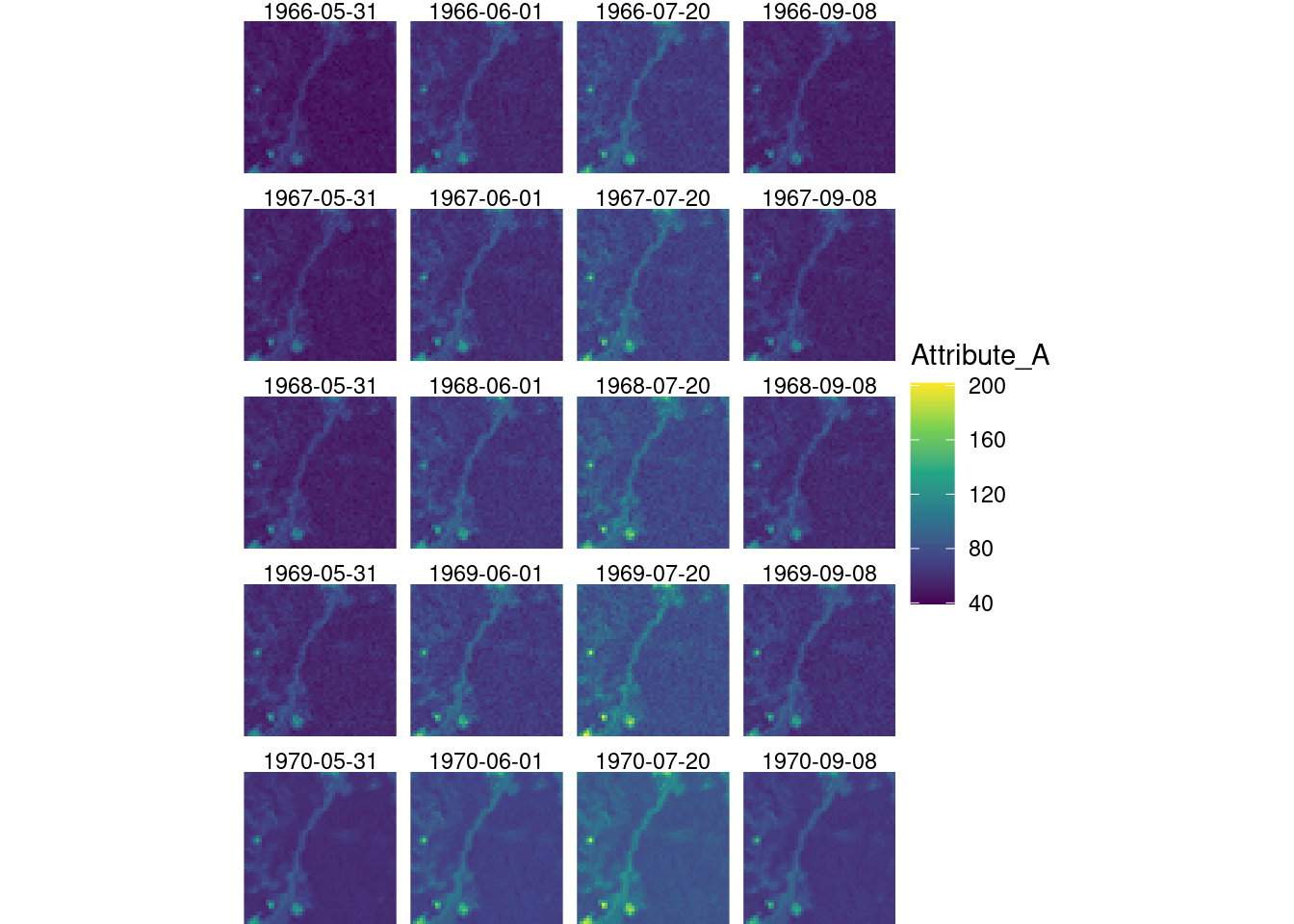
Saving these to file.
path <- "P:/41201785_okologisk_tilstand_2022_2023/data/climate_indicators/dummy_data"
saveRDS(y1, paste0(path, "/y1.rds"))
saveRDS(y2, paste0(path, "/y2.rds"))
saveRDS(y3, paste0(path, "/y3.rds"))
saveRDS(y4, paste0(path, "/y4.rds"))
saveRDS(y5, paste0(path, "/y5.rds"))
23.8.1.1.1 Dummy regions and ET map
Here is some dummy data for accounting areas (regions) and ecosystem occurrences as well, in case I need them later.
dummy_aa <- x %>%
  filter(time == oldTime[1]) %>%
  adrop() %>%
  mutate(accountingAreas = rep(c(1,2), each=length(Attribute_A)/2)) %>%
  select(accountingAreas)

tm_shape(dummy_aa) +
  tm_raster(style="cat")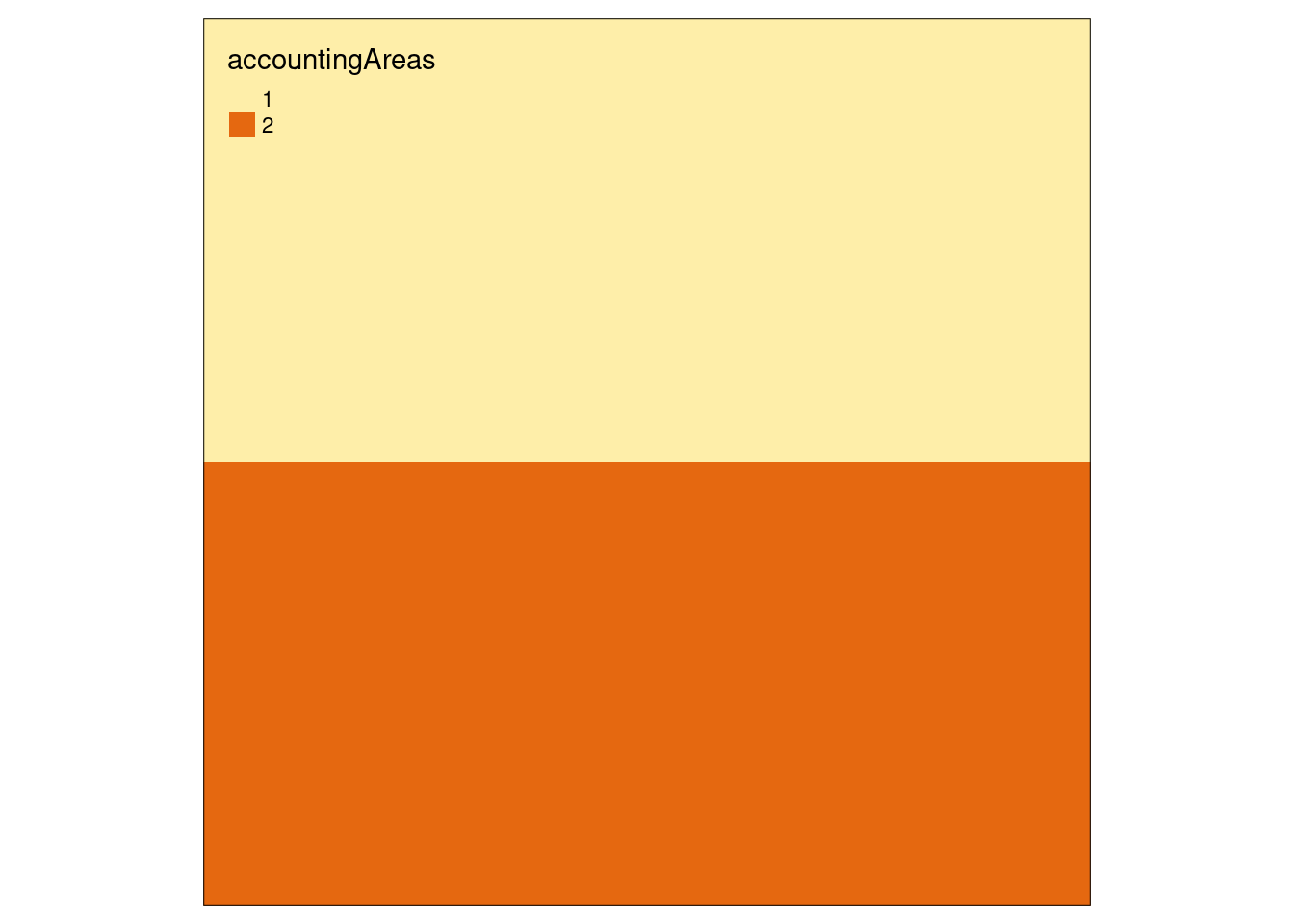
Figure 19.7: Showing the example account area delineation (raster format)
dummy_et <- x %>%
  filter(time == oldTime[1]) %>%
  adrop() %>%
  mutate(ecosystemType = rep(c(1,NA), length.out = length(Attribute_A))) %>%
  select(ecosystemType)

tm_shape(dummy_et) +
  tm_raster(style="cat")
Figure 23.1: Showing the example Ecosystem type delineation data.
23.8.1.2 Regions
Importing a shape file with the regional delineation.
reg <- sf::st_read("data/regions.shp", options = "ENCODING=UTF8")
#> options:        ENCODING=UTF8
#> Reading layer `regions' from data source
#>   `/data/Egenutvikling/41001581_egenutvikling_anders_kolstad/github/ecosystemCondition_v2/data/regions.shp'
#>   using driver `ESRI Shapefile'
#> Simple feature collection with 5 features and 2 fields
#> Geometry type: POLYGON
#> Dimension:     XY
#> Bounding box:  xmin: -99551.21 ymin: 6426048 xmax: 1121941 ymax: 7962744
#> Projected CRS: ETRS89 / UTM zone 33N
#st_crs(reg)
Outline of Norway
nor <- sf::st_read("data/outlineOfNorway_EPSG25833.shp")
#> Reading layer `outlineOfNorway_EPSG25833' from data source
#>   `/data/Egenutvikling/41001581_egenutvikling_anders_kolstad/github/ecosystemCondition_v2/data/outlineOfNorway_EPSG25833.shp'
#>   using driver `ESRI Shapefile'
#> Simple feature collection with 1 feature and 2 fields
#> Geometry type: MULTIPOLYGON
#> Dimension:     XY
#> Bounding box:  xmin: -113472.7 ymin: 6448359 xmax: 1114618 ymax: 7939917
#> Projected CRS: ETRS89 / UTM zone 33N
Remove marine areas from regions
reg <- st_intersection(reg, nor)
#> Warning: attribute variables are assumed to be spatially
#> constant throughout all geometries
tm_shape(reg) +
  tm_polygons(col="region")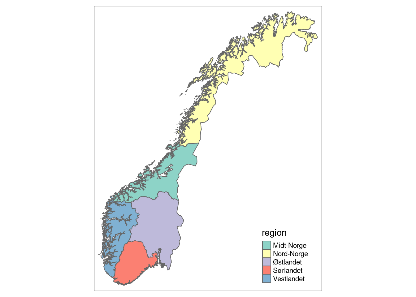
Figure 5.8: Five accounting areas (regions) in Norway.
23.8.2 Conceptual workflow
The general, the conceptual workflow is like this:
-
Collate variable data series
Import .nc files (loop though year 1961-1990) and subset to the correct attribute
Filter data by dates (optional) (
dplyr::filter). This means reading all 365 rasters into memory, and it is much quicker to filter out the correct rasters in the importing step above (see examples later in this chapter)Aggregate across time within a year (
stars::st_apply). This is the most time consuming operation in the workflow.Join all data into one data cube (
stars:c)
-
Calculate reference values
Aggregate (
st_apply)across reference years (dplyr::filter) to get median and sd valuesJoin with existing data cube (
stars:c)
-
Calculate indicator values
- Normalize climate variable at the individual grid cell level using the three reference values (
mutate(across()))
- Normalize climate variable at the individual grid cell level using the three reference values (
Mask by ecosystem type (This could also be done in step one, but it doesn’t speed things up to set some cells to NA)
-
Aggregate in space (to accounting areas) (zonal statistics)
Aggregate across 5 year time steps to smooth out random inter-annual variation and leave climate signal
Intersect with accounting area polygons
exactextrar::exact_extractand get mean/median and (spatial) sd. (Alternatively, get temporal sd at the grid cell level in the step above.)
Make trend figure and spatially aggregated maps,
23.8.4 Filter data by dates
Say we want to calculate the mean summer temperature. We then want to exclude the data for the times that is not withing our definition of summer.
Let’s try it on the dummy data. Remember this data had four time steps.
st_get_dimension_values(x, "time")
#> [1] "1970-05-31" "1970-06-01" "1970-07-20" "1970-09-08"
Our real data has 365 time steps for each year.
First I define my start and end dates. I want to keep only the summer data, defined as jun - aug.
start_month <-  "06"
end_month <- "08"
Then for each iteration I need to get the year as well
(year_temp <- year(st_get_dimension_values(x, "time")[1]))
#> [1] 1970
Then I can create a time interval object
start <- ym(paste(year_temp, start_month, sep="-"))
end <-  ym(paste(year_temp, end_month, sep="-"))
(myInterval <- interval(start, end))
#> [1] 1970-06-01 UTC--1970-08-01 UTC
Then I filter
x_aug <- x %>%
  select(Attribute_A) %>%
  adrop() %>%
  filter(time %within% myInterval)
st_get_dimension_values(x_aug, "time")
#> [1] "1970-06-01" "1970-07-20"
Later I discover that `dplyr::filter` work after reading the whole object to file, and therefor it is too slow for our use. I therefore filter data a different way further down.
23.8.5 Aggregate across time within a year
For this example I want to calculate the mean temperature over the summer. I therefore need to aggregate over time. Many climate indicators will need this functionality. There are two ways, either using st_apply or using aggregate.
temp_names <- year(st_get_dimension_values(x_aug, "time")[1])

microOut <- microbenchmark(
st_apply =  x_aug %>%
  st_apply(1:2, mean) %>%
  setNames(paste0("v_",temp_names)),
aggregate = x_aug %>%
  aggregate(by = "year", mean),
times=30
)
The time dimension is now gone as we have aggregated across it.
autoplot(microOut)
#> Coordinate system already present. Adding new coordinate
#> system, which will replace the existing one.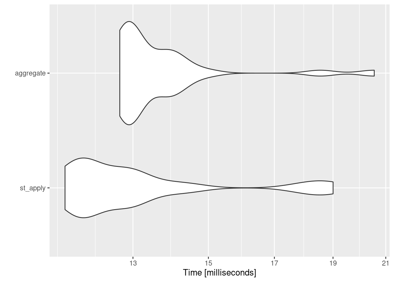
Figure 23.2: Comparing computation tome for two spatial aggregation functions.
st_apply is slightly faster, but aggregate has the advantage of that it retains the time dimension, whereas for st_apply I need to set the attribute name to be the year. I will try to use st_apply.
But let me see if I can save time by masking to ET before doing this operation.
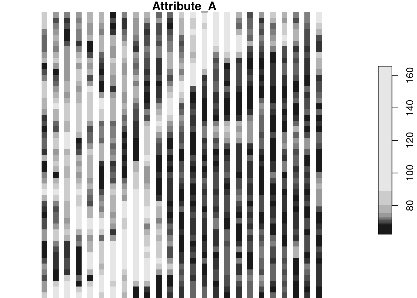
Figure 23.3: Demonstrating the effect of maskig the dummy data using a perfectly aligne raster ET map.
autoplot(
  microbenchmark(
No_masking =  x_aug %>%
  st_apply(1:2, mean) %>%
  setNames(paste0("v_",temp_names)),
Masking =  x_masked %>%
  st_apply(1:2, mean) %>%
  setNames(paste0("v_",temp_names))
 ), times=30
)
#> Coordinate system already present. Adding new coordinate
#> system, which will replace the existing one.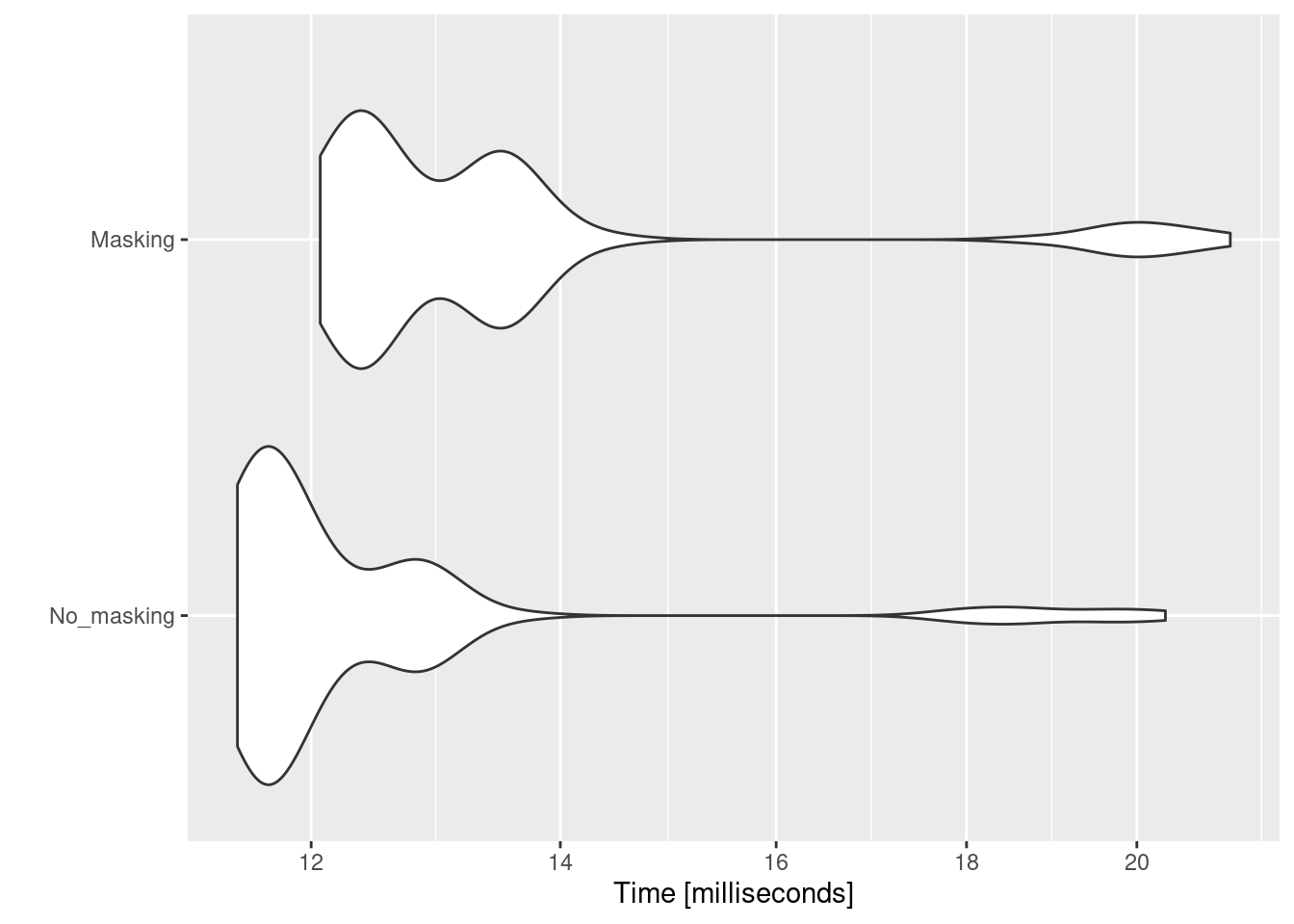
Figure 23.4: Comparing computation time before and after masking of raster data. There is no performance increase by masking before aggregating.
Since there is no increase in performance from masking, as we see in Fig. @ref(fig: withMasking) then it basically means we it is slower to mask beforehand, since the masking was not past of the benchmark assessment.
So, this is my solution:
# setNames dont work on stars proxy obejct, so I use rename instead
lookup <- setNames("mean", paste0("v_", temp_names))

x_summerMean <-   x_aug %>%
  st_apply(1:2, mean) %>%
  rename(all_of(lookup))
The v_ follows the naming convention we have developed for ourselves.
ggarrange(
ggplot() +
  geom_stars(data = x_aug) +
  coord_equal() +
  facet_wrap(~time) +
  theme_void() +
  scale_fill_viridis_c(option = "D") +  scale_x_discrete(expand = c(0, 0)) +
  scale_y_discrete(expand = c(0, 0)),


ggplot() +
  geom_stars(data = x_summerMean) +
  coord_equal() +
  #facet_wrap(~time) +
  theme_void() +
  scale_fill_viridis_c(option = "D") +
  scale_x_discrete(expand = c(0, 0)) +
  scale_y_discrete(expand = c(0, 0))
)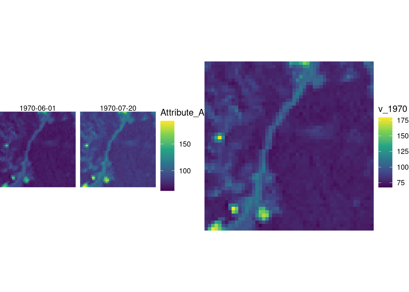
Figure 23.5: Plotting the dummy data showing Attribute_A for the two dates as small maps, and a larger map showing the mean for year 2018
Here’s the whole first step of the conceptual workflow in action, on the dummy data.
# Setting up the parameters
dir <- substr(getwd(), 1,2)
path <- ifelse(dir == "C:",
       "P:/",
       "/data/P-Prosjekter2/")
path2 <- paste0(path,
                "41201785_okologisk_tilstand_2022_2023/data/climate_indicators/dummy_data")
start_month <-  "06"
end_month <- "08"
myFiles <- list.files(path2, pattern=".rds", full.names = T)
summerTemp_fullSeries <- NULL

# Looping though the files in the directory
system.time({
for(i in 1:length(myFiles)){

  temp <- readRDS(myFiles[i]) %>%
    select(Attribute_A)

  year_temp <- year(st_get_dimension_values(temp, "time")[1])
  start <- ym(paste(year_temp, start_month, sep="-"))
  end <-  ym(paste(year_temp, end_month, sep="-"))
  myInterval <- interval(start, end)
  lookup <- setNames("mean", paste0("v_", year_temp))

  temp <- temp %>%
    filter(time %within% myInterval) %>%
    st_apply(1:2, mean) %>%
    rename(all_of(lookup))

  summerTemp_fullSeries <- c(temp, summerTemp_fullSeries)
  rm(temp) # same computation time with and without this function, but more tidy this way
}


# Turn the attributes into a dimension and rename the new attribute
summerTemp_fullSeries <- summerTemp_fullSeries %>%
  merge(name="Year") %>%
  setNames("Attribute_A")
})
#>    user  system elapsed
#>   0.134   0.000   0.141
And this is the result.
ggplot()+
  geom_stars(data = summerTemp_fullSeries) +
  coord_equal() +
  theme_void() +
  scale_fill_viridis_c(option = "D") +
  scale_x_discrete(expand = c(0, 0)) +
  scale_y_discrete(expand = c(0, 0))+
  facet_wrap(~Year)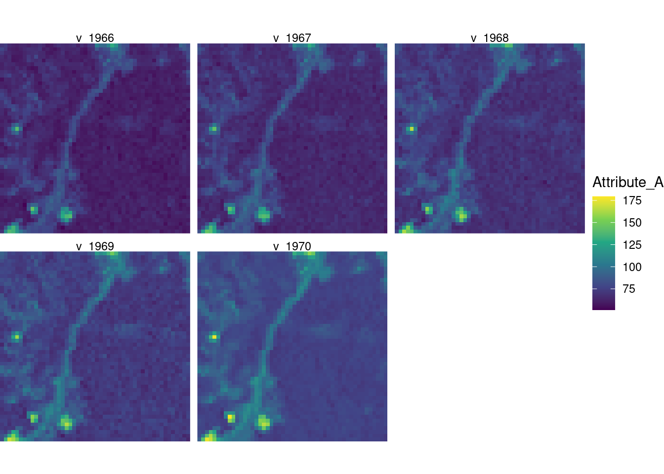
Figure 23.6: Temporal aggregation on the dummy data set.
Now let’s try it on the real data.
I initially tried to read stars proxy object and add steps to the call_list and execute these with st_as_stars, but this still returned proxy objects. Therefore I read the whole file in without proxy. To save time I can subset based on Julian dates.
I will use parallelization to speed things up.
path <- path <- ifelse(dir == "C:",
      "R:/",
      "/data/R/")

path2 <- paste0(path, "GeoSpatialData/Meteorology/Norway_SeNorge2018_v22.09/Original/rr_tm/")

myFiles <- list.files(path2, pattern=".nc$",full.names = T)
# The last file (the last year) is incomplete and don't include all julian dates that we select below, so I will not include it:
myFiles <- myFiles[-length(myFiles)]

real_temp_summer <- NULL

# set up parallel cluster using 10 cores
cl <- makeCluster(10L)

# Get julian days after defining months
temp <- stars::read_ncdf(paste(myFiles[1]), var="tg")
start_month_num <-  6
end_month_num <- 8

julian_start <- yday(st_get_dimension_values(temp, "time")[1] %m+%
                       months(+start_month_num))
julian_end <- yday(st_get_dimension_values(temp, "time")[1] %m+%
                     months(+end_month_num))
step <- julian_end-julian_start


for(i in 1:length(myFiles)){

  tic("init")
  temp <- stars::read_ncdf(paste(myFiles[i]), var="tg", proxy=F,
                           ncsub = cbind(start = c(1, 1, julian_start),
                              count = c(NA, NA, step)))
  year_temp <- year(st_get_dimension_values(temp, "time")[1])
  print(year_temp)
  lookup <- setNames("mean", paste0("v_", year_temp))
    # Perhaps leave out the v_ to get a numeric vector instead,
    # which is easier to subset
  st_crs(temp) <- 25833
  toc()

  tic("filter and st_apply")
  temp <- temp %>%
    #filter(time %within% myInterval) %>%
    st_apply(1:2, mean, CLUSTER = cl) %>%
    rename(all_of(lookup))
  toc()

  tic("c()")
  real_temp_summer <- c(temp, real_temp_summer)
  #rm(temp)
  toc()
}

tic("Merge")
real_temp_summer <- real_temp_summer %>%
  merge(name = "Year") %>%
  setNames("climate_variable")
toc()

stopCluster(cl)
This takes about 20 sec per file/year, or 22 min on total. That is not too bad. About 6000 raster are read into memory. Here’s a test for the effect of splitting over more cores.
cl <- makeCluster(2L)
cl2 <- makeCluster(6L)
cl3 <- makeCluster(10L)


tic("No cluster")
temp %>%
    #filter(time %within% myInterval) %>%
    st_apply(1:2, mean) %>%
    rename(all_of(lookup))
toc()

tic("Two clusters")
temp %>%
    #filter(time %within% myInterval) %>%
    st_apply(1:2, mean, CLUSTER = cl) %>%
    rename(all_of(lookup))
stopCluster(cl)
toc()

tic("Six clusters")
temp %>%
    #filter(time %within% myInterval) %>%
    st_apply(1:2, mean, CLUSTER = cl2) %>%
    rename(all_of(lookup))
stopCluster(cl2)
toc()

tic("Ten clusters")
temp %>%
    #filter(time %within% myInterval) %>%
    st_apply(1:2, mean, CLUSTER = cl3) %>%
    rename(all_of(lookup))
stopCluster(cl3)
toc()
No cluster: 21.401 sec elapsed
Two clusters: 21.546 sec elapsed
Six clusters: 14.548 sec elapsed
Ten clusters: 15.29 sec elapsed
Ten clusters (second run): 13.617 sec elapsed
The RStudio server has 48 cores. More parallel cores is probably on average faster. The NINA guidelines is to use max 10 cores, and to remember to close parallel cluster when done.
#saveRDS(real_temp_summer, "/data/P-Prosjekter2/41201785_okologisk_tilstand_2022_2023/data/climate_indicators/aggregated_climate_time_series/real_temp_summer.rds")
#write_stars(real_temp_summer, "/data/P-Prosjekter2/41201785_okologisk_tilstand_2022_2023/data/climate_indicators/aggregated_climate_time_series/real_temp_summer.tiff")
These files are about 500 MB, but the tiff file reads in a lot quicker then the rds file, so from now on I’ll just export as tiff. (This could perhaps have been solved with a gc(). Later I tried saving as RData with no speed issues problems, but then I had a problem with RData files seemingly becoming corrupted over time - stars objects saved as RData files would not bind together using c.stars() with other matching stars object and I think this could be related to a time stamp in the RData format. So, stick to tiff).
summer_median_temp <- read_stars(paste0(pData, "climate_indicators/aggregated_climate_time_series/real_temp_summer.tiff"),
                                 proxy=F)
names(summer_median_temp)
#> [1] "real_temp_summer.tiff"
dim(summer_median_temp)
#>    x    y band
#> 1195 1550   66
st_get_dimension_values(summer_median_temp, "Year")
#> NULL
Note that GTiff automatically renames the third dimension band and also renames the attribute.
st_get_dimension_values(summer_median_temp, "band")
#>  [1] "v_2022" "v_2021" "v_2020" "v_2019" "v_2018" "v_2017"
#>  [7] "v_2016" "v_2015" "v_2014" "v_2013" "v_2012" "v_2011"
#> [13] "v_2010" "v_2009" "v_2008" "v_2007" "v_2006" "v_2005"
#> [19] "v_2004" "v_2003" "v_2002" "v_2001" "v_2000" "v_1999"
#> [25] "v_1998" "v_1997" "v_1996" "v_1995" "v_1994" "v_1993"
#> [31] "v_1992" "v_1991" "v_1990" "v_1989" "v_1988" "v_1987"
#> [37] "v_1986" "v_1985" "v_1984" "v_1983" "v_1982" "v_1981"
#> [43] "v_1980" "v_1979" "v_1978" "v_1977" "v_1976" "v_1975"
#> [49] "v_1974" "v_1973" "v_1972" "v_1971" "v_1970" "v_1969"
#> [55] "v_1968" "v_1967" "v_1966" "v_1965" "v_1964" "v_1963"
#> [61] "v_1962" "v_1961" "v_1960" "v_1959" "v_1958" "v_1957"
I can rename them.
summer_median_temp <- summer_median_temp %>%
  st_set_dimensions(names = c("x", "y", "v_YEAR")) %>%
  setNames("temperature")
dim(summer_median_temp)
#>      x      y v_YEAR
#>   1195   1550     66
ggplot()+
  geom_stars(data = summer_median_temp[,,,c(1,11,22)], downsample = c(10, 10, 0)) +
  coord_equal() +
  theme_void() +
  scale_fill_viridis_c(option = "D") +
  scale_x_discrete(expand = c(0, 0)) +
  scale_y_discrete(expand = c(0, 0))+
  facet_wrap(~v_YEAR)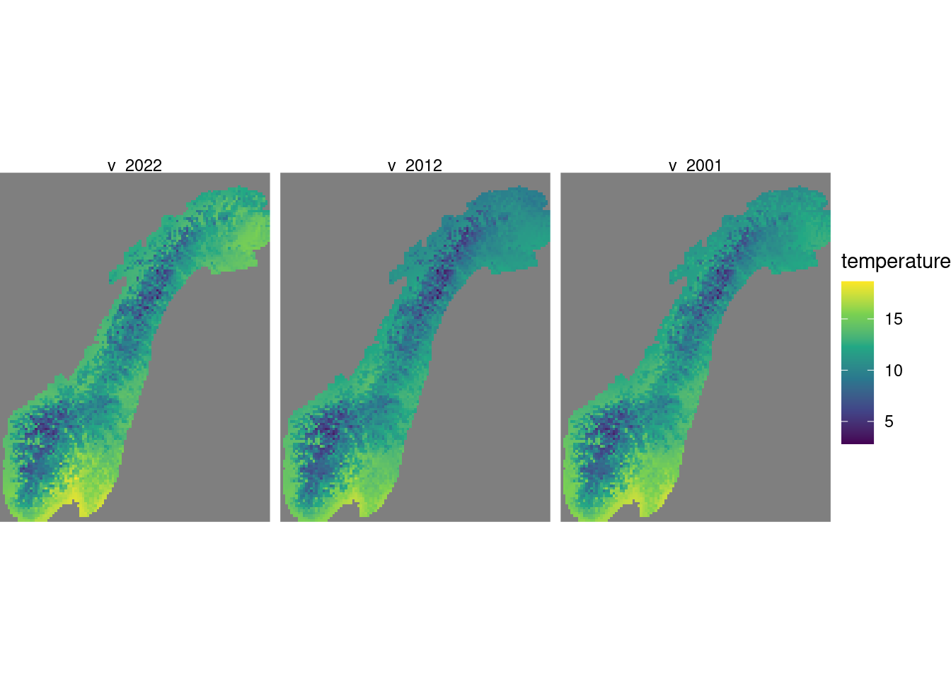
Figure 5.13: Showing three random slices of the year dimension.
23.8.6 Calculate reference values
23.8.6.1 Aggregate across reference years
We need to first to define a reference period and then to subset our data summer_median_temp. We can practice on the dummy data y.
dir <- substr(getwd(), 1,2)
path <- ifelse(dir == "C:",
       "P:/",
       "/data/P-Prosjekter2/")
path2 <- paste0(path,
                "41201785_okologisk_tilstand_2022_2023/data/climate_indicators/dummy_data")
myFiles <- list.files(path2, pattern=".rds", full.names = T)
y <- NULL

# Looping though the files in the directory
for(i in 1:length(myFiles)){
  temp <- readRDS(myFiles[i])
  y <- c(temp, y)
}
st_get_dimension_values(y, "time")
#>  [1] "1966-05-31" "1966-06-01" "1966-07-20" "1966-09-08"
#>  [5] "1967-05-31" "1967-06-01" "1967-07-20" "1967-09-08"
#>  [9] "1968-05-31" "1968-06-01" "1968-07-20" "1968-09-08"
#> [13] "1969-05-31" "1969-06-01" "1969-07-20" "1969-09-08"
#> [17] "1970-05-31" "1970-06-01" "1970-07-20" "1970-09-08"
y_filtered <- y %>%
  select(Attribute_A) %>%
  filter(time %within% interval("1961-01-01", "1990-12-31"))
Now we aggregate across years, again using st_apply.
dim(y_ref)
#> median_sd         x         y
#>         2        50        50
st_get_dimension_values(y_ref, "median_sd")
#> [1] "median" "sd"
It’s perhaps easier if median and sd are unique attributes, rather than levels of a dimension.
The attribute name mean we can change this to something more meaningful.
tmap_arrange(
tm_shape(y_ref)+
  tm_raster("reference_upper")
,
tm_shape(y_ref)+
  tm_raster("sd",
            palette = "-viridis")
)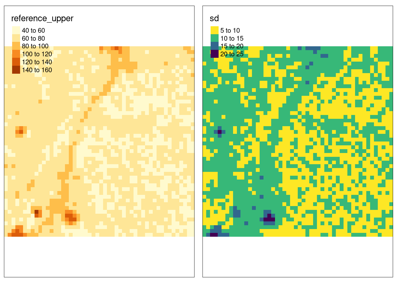
Figure 3.21: Showing the upper reference levels and the standard deviation from the dummy data set.
Let’s transfer this over to the real data. First we need to rename our dimension values and turn them back into dates.
new_dims <- as.Date(paste0(
  substr(st_get_dimension_values(summer_median_temp, "v_YEAR"), 3, 6), "-01-01"))
summer_median_temp_ref <- summer_median_temp %>%
  st_set_dimensions("v_YEAR", values = new_dims)
Then I can filter to leave only the reference period.
summer_median_temp_ref <- summer_median_temp_ref %>%
  filter(v_YEAR %within% interval("1961-01-01", "1990-12-31"))
st_get_dimension_values(summer_median_temp_ref, "v_YEAR")
#>  [1] "1990-01-01" "1989-01-01" "1988-01-01" "1987-01-01"
#>  [5] "1986-01-01" "1985-01-01" "1984-01-01" "1983-01-01"
#>  [9] "1982-01-01" "1981-01-01" "1980-01-01" "1979-01-01"
#> [13] "1978-01-01" "1977-01-01" "1976-01-01" "1975-01-01"
#> [17] "1974-01-01" "1973-01-01" "1972-01-01" "1971-01-01"
#> [21] "1970-01-01" "1969-01-01" "1968-01-01" "1967-01-01"
#> [25] "1966-01-01" "1965-01-01" "1964-01-01" "1963-01-01"
#> [29] "1962-01-01" "1961-01-01"
And then we calculate the median and sd like above
system.time({
cl <- makeCluster(10L)
summer_median_temp_ref <- summer_median_temp_ref %>%
  st_apply(c("x", "y"),
           FUN =  median_sd,
           CLUSTER = cl)
stopCluster(cl)
})| user | system | elapsed |
|---|---|---|
| 9.624 | 6.069 | 20.903 |
This is also something I can export.
# Note that write_stars can only export a single attribute, but we have put the 'attributes' as dimensions, and these will be read in as 'band' when importing tiff.
write_stars(summer_median_temp_ref, "/data/P-Prosjekter2/41201785_okologisk_tilstand_2022_2023/data/climate_indicators/aggregated_climate_time_series/summer_median_temp_ref.tiff")

# I initially saved as RData, like this, but ran into problems later when trying to bind stars objects using c.stars(). It appears RData becomes corrutpt in a sense, over time, perhaps due to some time stamp. If I recreated the object in the global environment and saved as RDatam I could read it in and work with it, but the next day it would not work again.
#saveRDS(summer_median_temp_ref, "/data/P-Prosjekter2/41201785_okologisk_tilstand_2022_2023/data/climate_indicators/aggregated_climate_time_series/summer_median_temp_ref.RData")
Pivot and turn dimension into attributes:
The attribute name is mean. We can change this to something more meaningful.
tmap_arrange(
tm_shape(st_downsample(summer_median_temp_ref_long, 10))+
  tm_raster("reference_upper")
,
tm_shape(st_downsample(summer_median_temp_ref_long, 10))+
  tm_raster("sd",
            palette = "-viridis")
)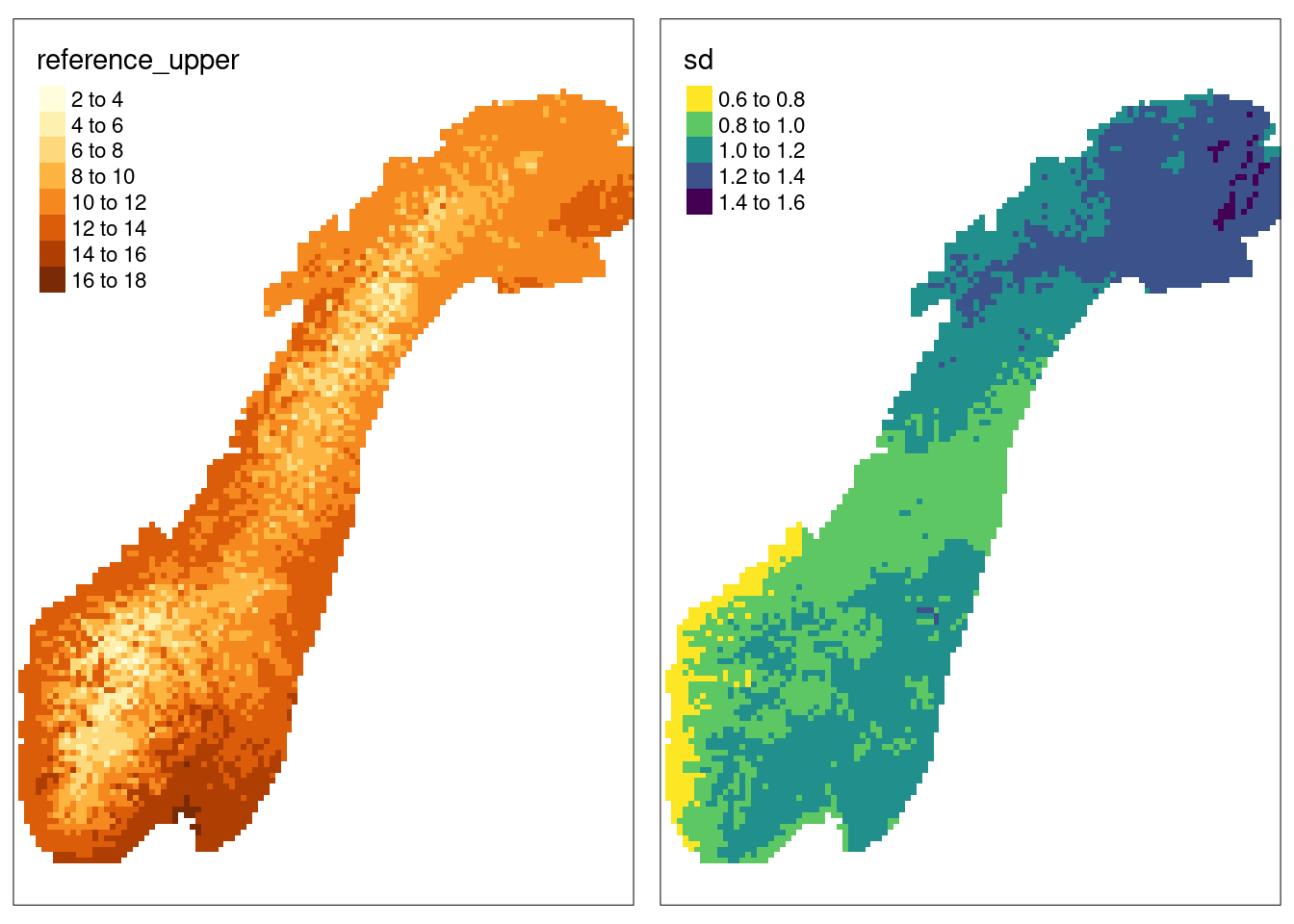
Figure 23.7: Showing the upper reference levels and the standard deviation from actual data of median summer temperatures.
23.8.7 Normalise variable
# select the columns to normalise
cols <- names(y_var)[!names(y_var) %in% c("reference_upper", "sd") ]
cols_new <- cols
names(cols_new) <- gsub("v_", "i_", cols)
# Mutate

# The break point scaling is actually not needed here, since
# having the lower ref value to be 5 sd implies that the threshold is
# 2 sd in a linear scaling.

system.time(
y_var_norm <- y_var %>%
  mutate(reference_low = reference_upper - 5*sd ) %>%
  mutate(reference_low2 = reference_upper + 5*sd ) %>%
  mutate(threshold_low = reference_upper -2*sd ) %>%
  mutate(threshold_high = reference_upper +2*sd ) %>%
  mutate(across(all_of(cols), ~
                  if_else(.x < reference_upper,
                  if_else(.x < threshold_low,
                                        (.x - reference_low) / (threshold_low - reference_low),
                                        (.x - threshold_low) / (reference_upper - threshold_low),
                                        ),
                  if_else(.x > threshold_high,
                                        (reference_low2 - .x) / (reference_low2 - threshold_high),
                                        (threshold_high - .x) / (threshold_high - reference_upper),
                                        )
                ))) %>%
  mutate(across(all_of(cols), ~ if_else(.x > 1, 1, .x))) %>%
  mutate(across(all_of(cols), ~ if_else(.x < 0, 0, .x))) %>%
  rename(all_of(cols_new)) %>%
  c(select(y_var, all_of(cols)))
)| user | system | elapsed |
|---|---|---|
| 14.803 | 2.717 | 17.512 |
Writing to file, this time as RData (could use rds) because tiff don’t allow multiple attributes, and because we don’t need to use c.stars() in this object.
gc()
saveRDS(y_var_norm, "/data/P-Prosjekter2/41201785_okologisk_tilstand_2022_2023/data/climate_indicators/aggregated_climate_time_series/summer_median_temp_normalised.RData")
lims <- c(-5, 22)

ggarrange(
ggplot() +
  geom_stars(data = st_downsample(y_var_norm["v_1970"],10)) +
  coord_equal() +
  theme_void() +
  scale_fill_viridis_c(option = "D",
                       limits = lims) +
  scale_x_discrete(expand = c(0, 0)) +
  scale_y_discrete(expand = c(0, 0))
,
ggplot() +
  geom_stars(data = st_downsample(y_var_norm["reference_upper"], 10)) +
  coord_equal() +
  theme_void() +
  scale_fill_viridis_c(option = "D",
                       limits = lims) +
  scale_x_discrete(expand = c(0, 0)) +
  scale_y_discrete(expand = c(0, 0))
,
ggplot() +
  geom_stars(data = st_downsample(y_var_norm["reference_low"], 10)) +
  coord_equal() +
  theme_void() +
  scale_fill_viridis_c(option = "D",
                       limits = lims) +
  scale_x_discrete(expand = c(0, 0)) +
  scale_y_discrete(expand = c(0, 0))
,

ggplot() +
  geom_stars(data = st_downsample(y_var_norm["reference_low2"], 10)) +
  coord_equal() +
  theme_void() +
  scale_fill_viridis_c(option = "D",
                       limits = lims) +
  scale_x_discrete(expand = c(0, 0)) +
  scale_y_discrete(expand = c(0, 0))
,

ggplot() +
  geom_stars(data = st_downsample(y_var_norm["i_1970"],10)) +
  coord_equal() +
  theme_void() +
  scale_fill_viridis_c(option = "A",
                       limits = c(0, 1)) +
  scale_x_discrete(expand = c(0, 0)) +
  scale_y_discrete(expand = c(0, 0))
, ncol=2, nrow=3, align = "hv"
)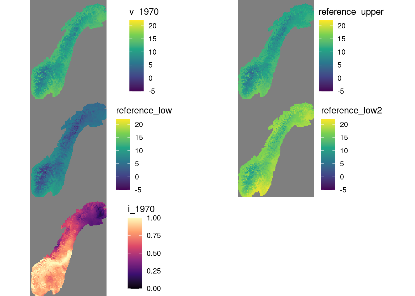
Figure 23.8: Example showing median summer tempretur in 1970, the upper and lwoer reference temperture, i.e. median and 5 SD units of the temperature between 1961-1990, and finally, the scaled indicator values.
The real indicator values should be means over 5 year periods. Calculating a running mean for all time steps is too time consuming. Therefore, the scaled, regional indicator values will be calculated for distinct time steps. The time series can perhaps best be presented with yearly resolution.
23.8.8 Plot time series as line graphs
We could also plot a time series as a series of maps, but then we need to average over these 5 year time periods first. We can get to that later.
To plot time series I first need to do a spatial aggregation. One option is to spatially aggregate the stars object directly, using the reg data set:
temp <- y_var_norm[1,,] %>%
  aggregate(reg, mean, na.rm=T)
plot(temp)
temp2 <- temp %>%
  st_as_sf() # too slow
However, this does no preserve the region name, and a subsequent st_intersection taks a little while and gives some boundary problems.
I can also convert pixels to points and then do the intersection.
temp_points <- y_var_norm[1,,] %>%
  st_as_sf(as_points = TRUE, merge = FALSE)
temp_points2 <- temp_points %>%
  st_intersection(reg) " too slow"
But this also took too long.
I can perhaps aggregate, and then turn to points and intersect, but that did not work perfect either.
I can rasterize the regions data set, turn it into a coded dimension and use st_apply, but that is tedious.
Let me try using exact_extract, as an alternative to aggregate. This requires us to turn to the terra package for a bit.
system.time(
regional_means <- rast(y_var_norm) %>%
  exact_extract(reg, fun = 'mean', append_cols = "region", progress=T) %>%
  setNames(c("region", names(y_var_norm)))
  )
user; system; elapsed: 7.603; 3.071; 10.697
That was fast!
I should also get the sd:
system.time(
regional_sd <- rast(y_var_norm) %>%
  exact_extract(reg, fun = 'stdev', append_cols = "region", progress=T) %>%
  setNames(c("region", names(y_var_norm)))
  )
user; system; elapsed: 7.420; 2.921; 10.355
Reshape and plot
div <- c("reference_upper",
         "reference_low",
         "reference_low2",
         "threshold_low",
         "threshold_high",
         "sd")

temp <- regional_means %>%
  as.data.frame() %>%
  select(region, div)

regional_means_long <- regional_means %>%
  as.data.frame() %>%
  select(!all_of(div)) %>%
  pivot_longer(!region) %>%
  separate(name, into=c("type", "year")) %>%
  pivot_wider(#id_cols = region,
              names_from = type)  %>%
  left_join(temp, by=join_by(region)) %>%
  mutate(diff = v-reference_upper) %>%
  mutate(threshold_low_centered = threshold_low-reference_upper) %>%
  mutate(threshold_high_centered = threshold_high-reference_upper)

#Adding the spatial sd
(
regional_means_long <- regional_sd %>%
  select(!all_of(div)) %>%
  pivot_longer(!region) %>%
  separate(name, into=c("type", "year")) %>%
  pivot_wider(names_from = type) %>%
  rename(i_sd = i,
         v_sd = v) %>%
  left_join(regional_means_long, by=join_by(region, year))
)
#> # A tibble: 330 × 15
#>    region     year   i_sd  v_sd     i     v reference_upper
#>    <chr>      <chr> <dbl> <dbl> <dbl> <dbl>           <dbl>
#>  1 Nord-Norge 2022  0.246  1.90 0.523  11.5            10.2
#>  2 Nord-Norge 2021  0.255  1.65 0.672  10.8            10.2
#>  3 Nord-Norge 2020  0.143  1.82 0.784  10.3            10.2
#>  4 Nord-Norge 2019  0.290  1.77 0.623  10.8            10.2
#>  5 Nord-Norge 2018  0.344  1.64 0.523  12.5            10.2
#>  6 Nord-Norge 2017  0.145  1.79 0.794  10.1            10.2
#>  7 Nord-Norge 2016  0.175  1.74 0.705  10.8            10.2
#>  8 Nord-Norge 2015  0.198  1.61 0.682  10.6            10.2
#>  9 Nord-Norge 2014  0.297  1.65 0.545  13.1            10.2
#> 10 Nord-Norge 2013  0.202  1.65 0.479  11.4            10.2
#> # ℹ 320 more rows
#> # ℹ 8 more variables: reference_low <dbl>,
#> #   reference_low2 <dbl>, threshold_low <dbl>,
#> #   threshold_high <dbl>, sd <dbl>, diff <dbl>,
#> #   threshold_low_centered <dbl>,
#> #   threshold_high_centered <dbl>
regOrder = c("Østlandet","Sørlandet","Vestlandet","Midt-Norge","Nord-Norge")

regional_means_long %>%
  mutate(col = if_else(diff>0, "1", "2")) %>%
  ggplot(aes(x = as.numeric(year),
           y = diff, fill = col))+
  geom_bar(stat="identity")+
  geom_hline(aes(yintercept = threshold_low_centered),
        linetype=2)+
  geom_hline(aes(yintercept = threshold_high_centered),
        linetype=2)+
  geom_segment(x = 1961, xend=1990,
               y = 0, yend = 0,
               linewidth=2)+
  scale_fill_hue(l=70, c=60)+
  theme_bw(base_size = 12)+
  ylab("Sommertempratur\navvik fra 1961-1990")+
  xlab("")+
  guides(fill="none")+
  facet_wrap( .~ factor(region, levels = regOrder),
              ncol=3,
              scales = "free_y")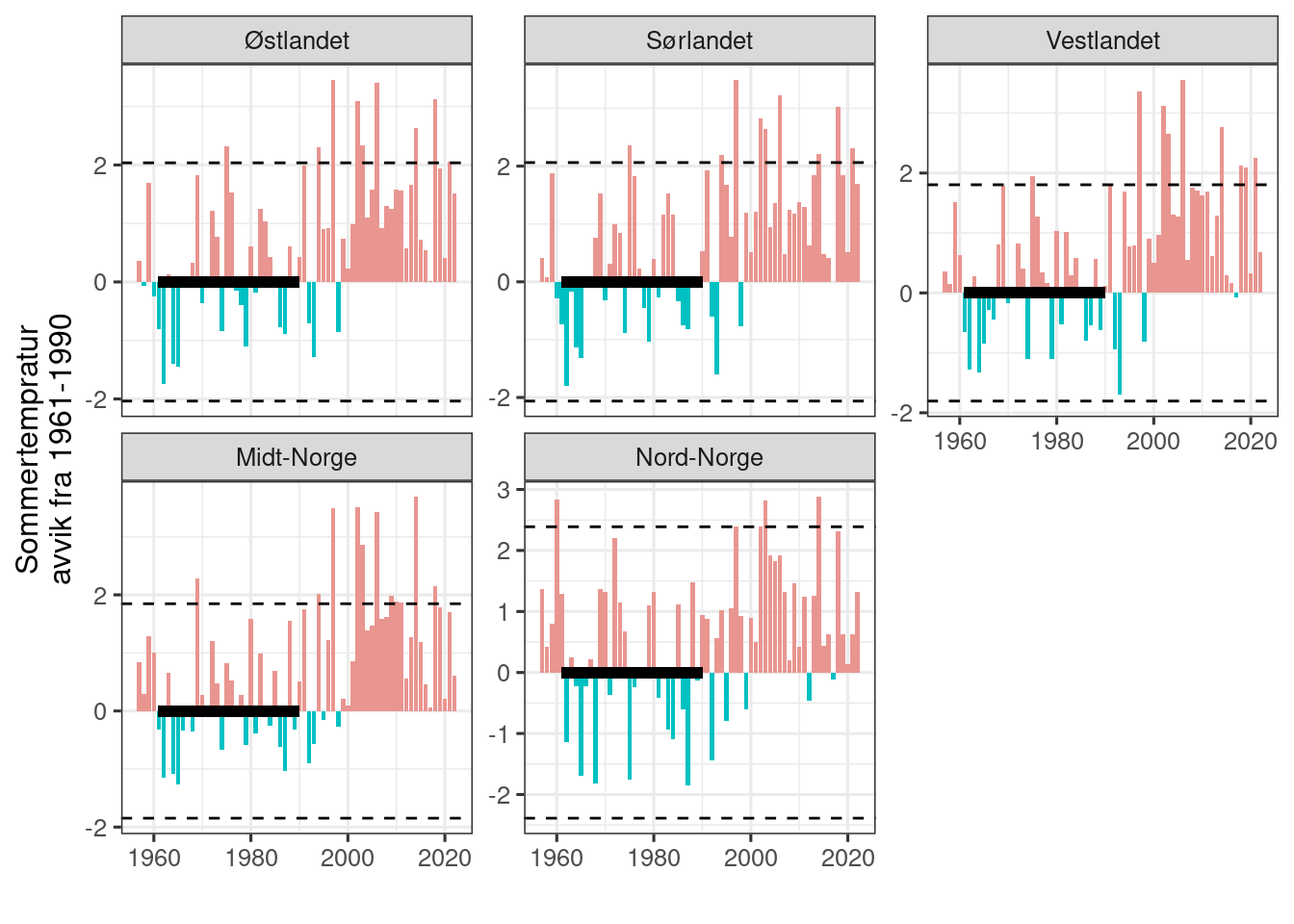
Figure 23.9: Times series for median summer temperature centered on the median value during the reference period. The reference period is indicated with a thick horizontal line. Dottet horisontal lines are 2 sd units for the reference period.
Then we can take the mean over the last 5 years and add to a spatial representation.
(
i_aggregatedToPeriods <- regional_means_long %>%
  mutate(year = as.numeric(year)) %>%
  mutate(period = case_when(
    year %between% c(2018, 2022) ~ "2018-2022",
    year %between% c(2013, 2017) ~ "2013-2017",
    year %between% c(2008, 2012) ~ "2008-2012",
    year %between% c(2003, 2007) ~ "2003-2007",
    .default = "pre 2003"
  )) %>%
  mutate(period_rank = case_when(
   period == "2018-2022" ~ 5,
   period == "2013-2017" ~ 4,
   period == "2008-2012" ~ 3,
   period == "2003-2007" ~ 2,
    .default = 1
  )) %>%
  group_by(region, period, period_rank) %>%
  summarise(indicator = mean(i),
            spatial_sd = sqrt(sum(i_sd^2))/length(i_sd)
            #,
            #spatial_sd_mean = mean(i_sd),
            #spatial_sd2_max = max(i_sd),
            #spatial_sd2_length = length(i_sd)
            )
)
#> `summarise()` has grouped output by 'region', 'period'. You
#> can override using the `.groups` argument.
#> # A tibble: 25 × 5
#> # Groups:   region, period [25]
#>    region     period    period_rank indicator spatial_sd
#>    <chr>      <chr>           <dbl>     <dbl>      <dbl>
#>  1 Midt-Norge 2003-2007           2     0.427     0.101
#>  2 Midt-Norge 2008-2012           3     0.573     0.143
#>  3 Midt-Norge 2013-2017           4     0.536     0.0986
#>  4 Midt-Norge 2018-2022           5     0.607     0.130
#>  5 Midt-Norge pre 2003            1     0.642     0.0277
#>  6 Nord-Norge 2003-2007           2     0.460     0.122
#>  7 Nord-Norge 2008-2012           3     0.675     0.109
#>  8 Nord-Norge 2013-2017           4     0.641     0.0937
#>  9 Nord-Norge 2018-2022           5     0.625     0.118
#> 10 Nord-Norge pre 2003            1     0.625     0.0266
#> # ℹ 15 more rows
labs <- unique(i_aggregatedToPeriods$period[order(i_aggregatedToPeriods$period_rank)])

i_aggregatedToPeriods %>%
  ggplot(aes(x = period_rank,
             y = indicator,
             colour=region))+
  geom_line() +
  geom_point() +
  geom_errorbar(aes(ymin=indicator-spatial_sd,
                    ymax=indicator+spatial_sd),
                    width=.2,
                 position=position_dodge(0.2)) +
  theme_bw(base_size = 12)+
  scale_x_continuous(breaks = 1:5,
                     labels = labs)+
  labs(x = "", y = "indikatorverdi")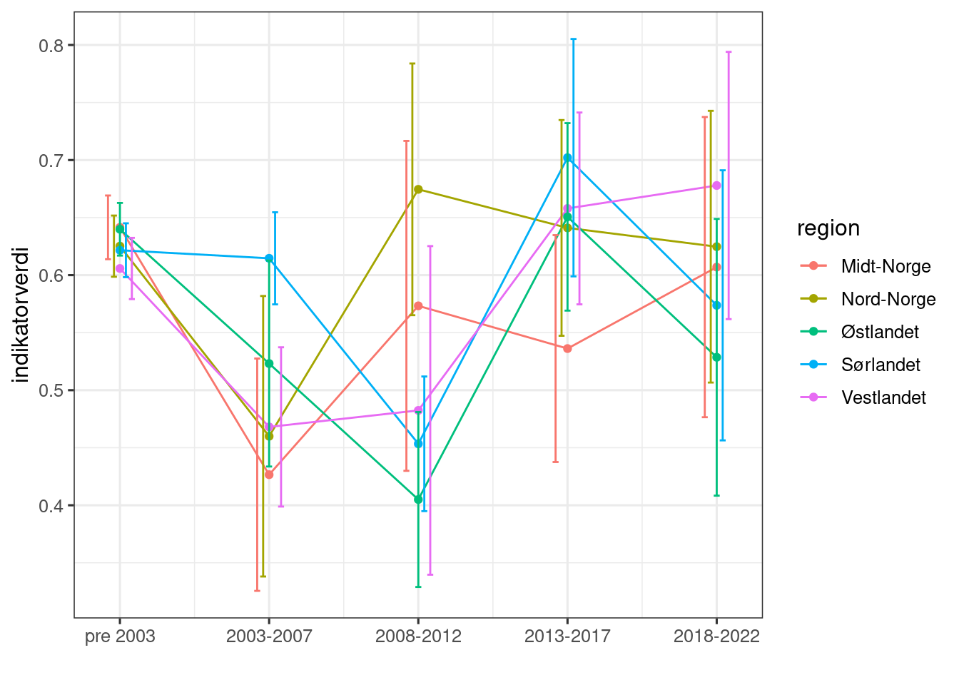
Figure 23.10: Scaled indicator values, aggregated over 5 year intervals. Errors represent spatial variation within regions and across years.
Finally, I can add these values to the sp object.
reg2 <- reg %>%
  left_join(i_aggregatedToPeriods[i_aggregatedToPeriods$period_rank==5,], by=join_by(region))
names(reg2)
#> [1] "id"          "region"      "GID_0"       "NAME_0"
#> [5] "period"      "period_rank" "indicator"   "spatial_sd"
#> [9] "geometry"
myCol <- "RdYlGn"
myCol2 <- "-RdYlGn"

tm_main <- tm_shape(reg2)+
  tm_polygons(col="indicator",
              title="Indikator:\nsommertemperatur",
    palette = myCol,
    style="fixed",
    breaks = seq(0,1,.2))

tm_inset <- tm_shape(reg2)+
  tm_polygons(col="spatial_sd",
              title="SD",
              palette = myCol2,
              style="cont")+
  tm_layout(legend.format = list(digits=2))

tmap_arrange(tm_main,
             tm_inset)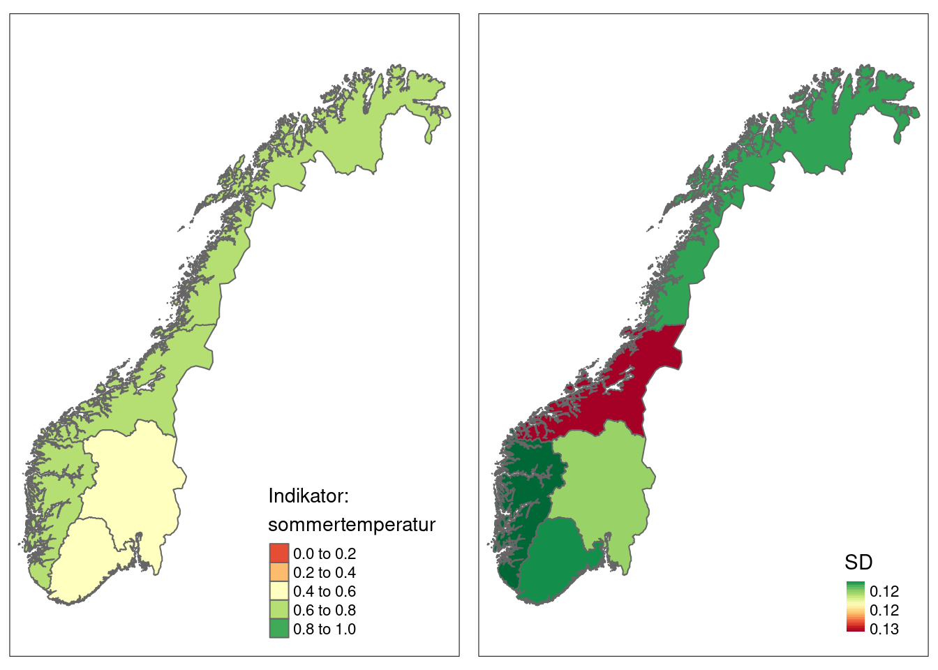
Figure 23.11: Summer tempreature indicator values for five accounting areas in Norway. SD is the spatial variation.