16 Flood frequency
Norwegian name: Oversvømmelseshyppighet
Author and date:
Vegar Bakkestuen
October 2023
Ecosystem |
Økologisk egenskap |
ECT class |
|---|---|---|
Våtmark |
Abiotiske forhold |
A1 Physical state characteristics |
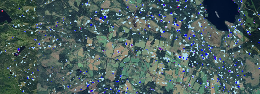
Figure 16.1: Flood frequency last 5 years, somewhere in Norway. Light blue areas are flooded once, and dark blue areas are flooded five times.
16.1 Introduction
Water and inundated areas is a land cover class that can be relatively easily distinguished from other land cover classes with high accuracy using remote sensing data, particularly Copernicus Sentinel-1 data. Sentinel-1 employs Synthetic Aperture Radar (SAR) instruments that can see through clouds. In Norway, Sentinel-1 data is available at a minimum frequency of once a week. Utilizing Google Earth Engine, all available Sentinel-1 data can be accessed, and there are pre-established scripts for distinguishing water-covered areas from other land cover classes. For example, you can refer to “Flood Mapping and Area Calculation of Flood Extent Using Sentinel-I SAR Data in Google Earth Engine:
“the case of Super Typhoon Odette (Rai)”, and;
“Applying Google Earth Engine for flood mapping and monitoring in the downstream provinces of the Mekong river”.
By aggregating Sentinel-1 images over an entire growing season, it becomes possible to model when areas are covered by water. This approach has been successfully used in various countries to map deltas and floodplains that are periodically submerged. We aim to apply this methodology to the deltas and floodplains in Norway to assess the accuracy of this method in Norwegian conditions. The code is developed in Java for Google Earth Engine and calculates flood frequency over a five-year period, which can be extended to ten years. Reference states need to be defined both before and after flood events, which is accomplished by specifying pre- and post-flood dates. You can determine these dates using hydrology scripts. This script uses Sentinel-1 imagery in a change detection approach, comparing images before and after a flood event. The key pre-processing steps for Sentinel-1 Ground Range Detected (GRD) data are thermal noise removal, radiometric calibration, and terrain correction. Therefore, the primary pre-processing step is applying a speckle filter. In this script, you can define your study area, select your desired time frame, and set SAR parameters. Make sure to adjust these parameters according to your study area’s specific conditions.
Workflow:
Calculate Flood Indicator Using Google Earth Engine Script
-
Initialization:
• Set up your Google Earth Engine environment.
• Import the necessary geometries or AOI.
-
Define Functions:
• Define a function for calculating flood extent and area based on the provided script. The function should take parameters like the year, polarization, and AOI.
-
Define Constants:
• Set constant values such as polarization, pass direction, smoothing radius, and difference threshold. Ensure these values are appropriate for your study area.
-
Define Years and Date Ranges:
• Create an array or list of years for which you want to calculate the flood indicator.
• Define the “before” and “after” date ranges for each year based on your specific study periods.
-
Loop Through Years:
• Use a loop to iterate through each year in your defined list.
• For each year, call the flood extent calculation function you defined, passing the appropriate parameters (e.g., SAR collections for “before” and “after,” polarization, AOI).
-
Calculate Flood Frequency:
• After calculating flood extent for each year, calculate the flood frequency. You can create a frequency count image by accumulating flood extent layers from each year.
-
Data Visualization:
• Define a color palette for displaying flood frequency on the map.
• Add the flood frequency layer to the map for visualization.
• Optionally, you can also display individual flood extents for each year.
-
Print Results:
• In the loop, after calculating flood extent for each year, print the calculated flood extent areas to the console for each year.
-
Data Export (Optional):
• If needed, you can export the results, such as the frequency map, for further analysis or reporting.
-
Fine-Tuning:
• As needed, adjust parameters in the script, such as smoothing radius, difference threshold, or additional data sources, to optimize the flood indicator calculation.
-
Interpretation:
• Analyze the results to understand the flood extent areas and frequencies for different years.
16.2 About the underlying data
The flood frequency indicator is derived from a time series of Sentinel-1 SAR data covering multiple years. The analysis involves the following steps:
- Data Collection: Sentinel-1 GRD imagery, including the VH polarization, was used to create a comprehensive dataset. The data covered several years, enabling a temporal perspective on flood frequency.
- Preprocessing: The data underwent preprocessing, including thermal-noise removal, radiometric calibration, and terrain correction, resulting in high-quality radar backscatter information. A speckle filter was applied for data refinement.
- Flood Extent Calculation: Flood extents for each year were determined through a change detection approach, comparing “before” and “after” flood event images. The selected polarization, VH, was utilized to differentiate flooded areas.
- Flood Frequency Mapping: The accumulated flood extents for different years were used to create a flood frequency map. This map illustrates the frequency of flooding events in the study area over the analyzed period.
16.2.1 Representativity in time and space
The analysis spans multiple years, offering a long-term view of flooding events in the study area. This extended time frame enables the identification of recurrent patterns and trends, which is vital for understanding wetland dynamics.
16.2.4 Aditional comments about the dataset
Sentinel-1 data provides valuable information; however, its spatial and temporal resolution can affect the accuracy of flood extent mapping. In this analysis, a 10-meter spatial resolution was used, which means that smaller-scale features may not be fully captured. Additionally, Sentinel-1 data has a temporal revisit time, which may result in missed flood events or difficulties in distinguishing between different flood events that occurred close in time.
16.3 Ecosystem characteristic
In the context of the Norwegian standard, the ‘Flood frequency’ indicator aligns with the ecosystem characteristic known as Abiotiske forhold. Flood frequency is a crucial factor in understanding how changes in hydrology, including flood events, influence the composition and distribution of species within ecosystems. It can also be instrumental in evaluating the resilience of ecosystems to such disturbances.
Furthermore, the indicator could also be relevant in the context of ‘funksjonelt viktige arter og strukturer,’ or ‘functionally important species and structures.’ Flood frequency plays a pivotal role in shaping the habitat availability and accessibility for species critical to ecosystem functioning. This includes species that are essential for nutrient cycling, species recruitment, and other key ecosystem functions. Frequent or infrequent flood events can have far-reaching consequences on the viability of these functionally important components of ecosystems.
Therefore, understanding and monitoring flood frequency not only serve as a hydrological metric but also have profound implications for ecosystem dynamics, which are vital for the overall health and sustainability of ecosystems. This integrated perspective highlights the interconnectedness of hydrological patterns and ecosystem characteristics, emphasizing the indicator’s significance in ecological and conservation assessments.
16.4 Collinearities with other indicators
Flood frequency is not thought to exhibit collinearity with any other indicator at the present.
16.5 Reference condition and values
16.5.1 Reference condition
The reference condition is one where human activities that impact large scale hydrological patterns are minimal. The most important drivers of anthropogenic change are climate change, water regulation, draning and flood prevention and river channelization.
16.5.2 Reference values, thresholds for defining good ecological condition, minimum and/or maximum values
Reference values are not yet developed for this indicator. Note that the term reference level when used for this indicator sometime pertains to baseline hydrological conditions, and not a reference for the level of flood frequency under the reference condition.
16.7 Analyses
16.7.1 NVE data
Innsynsløsning: https://nina.maps.arcgis.com/apps/instant/basic/index.html?appid=4344dd7f769048ed9dedf1803638ff48
Baseline data for hydrological parameters, such as water level, water flow, and temperature, are crucial for assessing the ecological condition of aquatic ecosystems. In the context of this analysis, we are planning to derive baseline values from extensive datasets collected by the Norwegian Water Resources and Energy Directorate (NVE) through its hydrological API (HydAPI). NVE has been instrumental in gathering long-term hydrological data, with records dating back to the 1800s. These historical measurements serve as a valuable baseline to evaluate contemporary conditions.
W Data Retrieval Solution - Python Code (get-observations-NINA.py):
This Python script (get-observations-NINA.py) serves as a data retrieval solution to access hydrological data from the Norwegian Water Resources and Energy Directorate’s (NVE) Hydrological API (HydAPI). It is designed to fetch observational data and metadata for hydrological stations across Norway. The script is versatile and allows users to specify parameters such as the station ID, observed parameters, resolution time, reference time, and a mandatory API key.
• Station ID (-s): Users can input one or multiple station IDs separated by a comma, allowing access to specific hydrological data from various locations.
• Parameters (-p): This parameter allows users to specify the type of observation data they need. Multiple parameters can be specified, enhancing flexibility.
• Resolution Time (-r): Users can select the resolution time, choosing between instantaneous (0), hourly (60), or daily (1440) data.
• API Key (-a): The API key is a mandatory component to authenticate and access the HydAPI data. Users need to register and obtain their API key from the HydAPI platform.
The script leverages Python’s request library to send HTTP requests to the HydAPI, and it retrieves data in JSON format. It also provides the ability to define a reference time for data retrieval. The retrieved data is written to a user-defined output file, facilitating further analysis and utilization.
Data Retrieval Procedure:
To retrieve data using the code:
- Set Working Directory: Define the desired folder path, typically using the os.chdir() function, to ensure that the script operates in the intended directory.
- Define the Command: Create a command as a list of strings, including the Python interpreter (python), the script name (get-observations-NINA.py), and the various parameters required for data retrieval (e.g., station, parameters, resolution time, and API key).
- Execute the Command: Use subprocess.call() to execute the command, which triggers the Python script to fetch the requested data from the HydAPI.
- Data Output: The retrieved data is written to a JSON file named according to the station, e.g., output_file = r’C:_xxx.json’.
Script (in python)
Koden er skrevet i python og henter hydrologiske data fra NVE sin API. Skriptet heter get-observations-NINA.py. Den fungerer hvis man oppretter en mappe på C:/ kalt Konnektivetet/python og legger scriptet der.
#!/usr/bin/python

import getopt
import json
import sys

try:
    from urllib.request import Request, urlopen  # Python 3
except ImportError:
    from urllib2 import Request, urlopen  # Python 2


def usage():
    print()
    print("Get observations from the NVE Hydrological API (HydAPI)")
    print("Parameters:")
    print("   -a: ApiKey (mandatory). ")
    print("   -s: StationId (mandatory). Several stations can be given separated by a comma. Example \"6.10.0,12.209.0\"")
    print("   -p: Parameter (mandatory). Several Parameters can be given separated by a comma.")
    print("   -r: Resolution time. 0 (instantaneous), 60 (hourly), or 1440 (daily). (mandatory)")
    print("   -t: Reference time. See documentation for reference time. Example \"P1D/\", gives one day back in time. If none given, the last observed value will be returned")
    print("   -h: This help")
    print()
    print("Example:")
    print("    python get-observations.py -a \"INSERT_APIKEY_HERE\" -s \"6.10.0,12.209.0\" -p \"1000,1001\" -r 60 -t \"P1D/\"")
    print()


def main(argv):
    try:
        opts, args = getopt.getopt(argv, "a:s:p:r:ht:")
    except getopt.GetoptError as err:
        print(str(err))  # will print something like "option -a not recognized"
        usage()
        sys.exit(2)

    station = None
    parameter = None
    resolution_time = None
    api_key = None
    reference_time = None

    for opt, arg in opts:
        if opt == "-s":
            station = arg
        elif opt == "-p":
            parameter = arg
        elif opt == "-r":
            resolution_time = arg
        elif opt == "-a":
            api_key = arg
        elif opt == "-t":
            reference_time = arg
        elif opt == "-h":
            usage()
            sys.exit()
        else:
            assert False, "unhandled option"

    if api_key is None:
        print("Error: You must supply the API key with your request (-a)")
        usage()
        sys.exit(2)

    if station is None or parameter is None or resolution_time is None:
        print("Error: You must supply the parameters station (-s), parameter (-p), and resolution time (-r)")
        usage()
        sys.exit(2)

    baseurl = "https://hydapi.nve.no/api/v1/Observations?StationId={station}&Parameter={parameter}&ResolutionTime={resolution_time}"

    url = baseurl.format(station=station, parameter=parameter, resolution_time=resolution_time)

    if reference_time is not None:
        url = "{url}&ReferenceTime={reference_time}".format(url=url, reference_time=reference_time)

    print(url)

    request_headers = {
        "Accept": "application/json",
        "X-API-Key": api_key
    }

    request = Request(url, headers=request_headers)

    response = urlopen(request)
    content = response.read().decode('utf-8')

    output_file = r'C:\Konnektivitet\Stasjon_xxx.json'  # Definerer stien til utdatafilen

    with open(output_file, 'w') as outfile:
        outfile.write(content)

    print(f"Data written to {output_file}")


if __name__ == "__main__":
    main(sys.argv[1:])
Dataene hentes ut ved å skrive inn følgende kommandoer i python vinduet:
import os
#Angi banen til den ønskede mappen
ny_mappe = r'C:\Konnektivitet\python'
Endre den aktive mappen til den nye mappen
os.chdir(ny_mappe)

import subprocess
# Definer kommandoen som en liste av strenger
kommando = [
     'python',                # Dette er kommandoen du vil kjøre (Python)
     'get-observations-NINA.py',   # Dette er navnet på Python-skriptet du vil kjøre
     '-a', '4B2BQZYxbEiommYw8YCB8w==', # Mulig alle må lage sin egen API key: hydapi.nve.no/Users
     '-s', '12.209.0', # Dette er stasjonsnummer som kan hentes fra NINA innsynsløsning (se under).
     '-p', '1000', # spesifikk type observasjon – se hydapi.nve.no/UserDocumentation/
     '-r', '60', # oppløsningstid. 60 indikerer en times oppløsning
     '-t', '2018-01-01T10:00:00/2018-01-14T20:00:00'  # Merk at timestamp er uten ekstra anførselstegn
 ]
subprocess.call(kommando)
Sentinel-1 radar data can be affected by speckle noise, which appears as random variations in pixel values. While speckle filtering was applied to reduce this noise, some level of uncertainty remains, particularly in areas with complex terrain.
16.8 JAVA code
You must run the whole code below. There is a maximum of 5000 wetland polygons for each export.
/*===========================================================================================
                       SAR-FLOOD MAPPING USING A CHANGE DETECTION APPROACH
  ===========================================================================================
  This script uses Sentinel-1 SAR data to create a flood extent map. It employs a change
  detection method, comparing before- and after-flood images. The script is designed to work
  with Ground Range Detected (GRD) imagery, which undergoes preprocessing steps, including
  Thermal-Noise Removal, Radiometric Calibration, and Terrain Correction. Therefore, only a
  Speckle filter needs to be applied during preprocessing.

  ===========================================================================================

                                  SELECT YOUR OWN STUDY AREA

   Use the polygon tool in the top left corner of the map pane to outline your study area.
   Single clicks add vertices, and double-clicking completes the polygon.
   **CAUTION**: Under 'Geometry Imports' (top left in the map panel), uncheck the
               geometry box to avoid obscuring the view of the imagery later.

  *******************************************************************************************
                                       SET TIME FRAME

   Specify the start and end dates for a period BEFORE the flood event. Ensure that the
   duration is sufficient for Sentinel-1 to acquire images (repetition rate = 6 days).
   Adjust these parameters if the ImageCollections (see Console) are empty.

/********************************************************************************************
                           SET SAR PARAMETERS (can be left default)*/

var polarization = "VH"; /* or 'VV' --> VH is commonly preferred for flood mapping, but
                           the choice may depend on your study area. You can choose 'VV' as
                           well. */

var pass_direction = "DESCENDING"; /* or 'ASCENDING'. When comparing images, use only one
                           pass direction. Consider changing this parameter if your image
                           collection is empty. In some areas, more Ascending images exist
                           than Descending, or vice versa. */

var difference_threshold = 1.25; /* Threshold applied to the difference image (after flood
                           - before flood). The value is chosen through trial and error.
                           If your flood extent result contains many false positives or
                           negatives, consider adjusting it. */
//var relative_orbit = 79;
                          /* If you know the relative orbit for your study area, you can
                           filter your image collection by it here to avoid errors due to
                           comparisons across different relative orbits. */

/********************************************************************************************
  ---->>> DO NOT EDIT THE SCRIPT PAST THIS POINT! (unless you know what you are doing) <<<---
  ------------------>>> now hit the 'RUN' at the top of the script! <<<-----------------------
  -----> The final flood product will be ready for download on the right (under tasks) <-----
  ******************************************************************************************/

//---------------------------------- Translating User Inputs ------------------------------//
Map.setCenter(9.98383,  60.95329, 14); // Sets the map center.

var before_start = '2023-04-01';
var before_end = '2023-07-01';
// Define the start and end dates for the period before the flood.

var after_start = '2023-08-01';
var after_end = '2023-08-25';
// Define the start and end dates for the period after the flood.

//------------------------------- DATA SELECTION & PREPROCESSING --------------------------//

// Rename the selected geometry feature
var aoi = ee.FeatureCollection(geometry);

// Load and filter Sentinel-1 GRD data based on predefined parameters
var collection = ee.ImageCollection('COPERNICUS/S1_GRD')
  .filter(ee.Filter.eq('instrumentMode', 'IW'))
  .filter(ee.Filter.listContains('transmitterReceiverPolarisation', polarization))
  .filter(ee.Filter.eq('orbitProperties_pass', pass_direction))
  .filter(ee.Filter.eq('resolution_meters', 10))
  //.filter(ee.Filter.eq('relativeOrbitNumber_start', relative_orbit ))
  .filterBounds(aoi)
  .select(polarization);

// Select images based on predefined dates
var before_collection = collection.filterDate(before_start, before_end);
var after_collection = collection.filterDate(after_start, after_end);

// Print selected tiles to the console
function dates(imgcol) {
    var range = imgcol.reduceColumns(ee.Reducer.minMax(), ["system:time_start"]);
    var printed = ee.String('from ')
      .cat(ee.Date(range.get('min')).format('YYYY-MM-dd'))
      .cat(' to ')
      .cat(ee.Date(range.get('max')).format('YYYY-MM-dd'));
    return printed;
}

var before_count = before_collection.size();
print(ee.String('Tiles selected: Before Flood ').cat('(').cat(before_count).cat(')'),
    dates(before_collection), before_collection);

var after_count = before_collection.size();
print(ee.String('Tiles selected: After Flood ').cat('(').cat(after_count).cat(')'),
    dates(after_collection), after_collection);

// Create a mosaic of selected tiles and clip to the study area
var before = before_collection.mosaic().clip(aoi);
var after = after_collection.mosaic().clip(aoi);

// Apply radar speckle reduction by smoothing
var smoothing_radius = 50;
var before_filtered = before.focal_mean(smoothing_radius, 'circle', 'meters');
var after_filtered = after.focal_mean(smoothing_radius, 'circle', 'meters');

//------------------------------- FLOOD EXTENT CALCULATION -------------------------------//
// Calculate the difference between the before and after images
var difference = after_filtered.divide(before_filtered);

//Map.addLayer(difference, {}, 'Difference 2023', 1);

// Apply the predefined difference threshold to create the flood extent mask
var threshold = difference_threshold;
var difference_binary = difference.gt(threshold);

// Refine the flood result using additional datasets
// Include the JRC layer on surface water seasonality to mask flood pixels from areas
// with "permanent" water (water > 10 months of the year)
var swater = ee.Image('JRC/GSW1_0/GlobalSurfaceWater').select('seasonality');
var swater_mask = swater.gte(10).updateMask(swater.gte(10));

// Create a flooded mask where perennial water bodies (water > 10 mo/yr) are assigned a 0 value
var flooded_mask = difference_binary.where(swater_mask, 0);
// Create the final flooded area without pixels in perennial water bodies
var flooded = flooded_mask.updateMask(flooded_mask);

// Compute the connectivity of pixels to eliminate those connected to 8 or fewer neighbors
// This operation reduces noise in the flood extent product
var connections = flooded.connectedPixelCount();
var flooded = flooded.updateMask(connections.gte(8));

// Mask out areas with more than 5 percent slope using the Norwegian Digital Elevation Model
//var DEM = ee.Image('WWF/HydroSHEDS/03VFDEM');
var DEM = ee.Image('users/vegar/dem_10m_kartverket');
var terrain = ee.Algorithms.Terrain(DEM);
var slope = terrain.select('slope');
var flooded = flooded.updateMask(slope.lt(5));

// Calculate flood extent area
// Create a raster layer containing the area information of each pixel
var flood_pixelarea = flooded.select(polarization)
  .multiply(ee.Image.pixelArea());

// Sum the areas of flooded pixels
// The default 'bestEffort' is set to true to reduce computation time; for a more
// accurate result, set 'bestEffort' to false and increase 'maxPixels'.
var flood_stats = flood_pixelarea.reduceRegion({
  reducer: ee.Reducer.sum(),
  geometry: aoi,
  scale: 10, // native resolution
  //maxPixels: 1e9,
  bestEffort: true
});

// Convert the flood extent to hectares (area calculations are originally given in meters)
var flood_area_ha = flood_stats
  .getNumber(polarization)
  .divide(10000)
  .round();

// Set visualization parameters
var frequencyVis = {
  min: 0,
  max: 4,
  palette: ['white', 'lightblue', 'mediumblue', 'darkblue', 'black']
};

// Display flooded areas
Map.addLayer(flooded, { palette: "0000FF" }, 'Flooded areas Hans 2023', 0);

//----------------------------- Compare with the previous year 2022------------------------

var before_start2 = '2022-04-01';
var before_end2 = '2022-09-01';

var after_start2 = '2023-08-01'; // Should match the reference state
var after_end2 = '2023-08-25'; // Should match the reference state

var before_collection2 = collection.filterDate(before_start2, before_end2);
var after_collection2 = collection.filterDate(after_start2, after_end2);

// Create a mosaic of selected tiles and clip to the study area
var before2 = before_collection2.mosaic().clip(aoi);
var after2 = after_collection2.mosaic().clip(aoi);

// Apply radar speckle reduction by smoothing
var smoothing_radius = 50;
var before_filtered2 = before2.focal_mean(smoothing_radius, 'circle', 'meters');
var after_filtered2 = after2.focal_mean(smoothing_radius, 'circle', 'meters');

// Calculate the difference between the before and after images
var difference2 = after_filtered2.divide(before_filtered2);

// Apply the predefined difference-threshold and create the flood extent mask
var threshold2 = difference_threshold;
var difference_binary2 = difference2.gt(threshold2);

// Refine the flood result using additional datasets
// Include the JRC layer on surface water seasonality to mask flood pixels from areas
// with "permanent" water (water > 10 months of the year)
var swater = ee.Image('JRC/GSW1_0/GlobalSurfaceWater').select('seasonality');
var swater_mask = swater.gte(10).updateMask(swater.gte(10));

// Create a flooded mask where perennial water bodies (water > 10 mo/yr) are assigned a 0 value
var flooded_mask2 = difference_binary2.where(swater_mask, 0);
// Create the final flooded area without pixels in perennial water bodies
var flooded2 = flooded_mask2.updateMask(flooded_mask2);

// Compute the connectivity of pixels to eliminate those connected to 8 or fewer neighbors
// This operation reduces noise in the flood extent product
var connections2 = flooded2.connectedPixelCount();
var flooded2 = flooded2.updateMask(connections2.gte(8));

// Mask out areas with more than 5 percent slope using a Digital Elevation Model
var DEM = ee.Image('users/vegar/dem_10m_kartverket');
var terrain = ee.Algorithms.Terrain(DEM);
var slope = terrain.select('slope');
flooded2 = flooded2.updateMask(slope.lt(5));

// Calculate flood extent area
// Create a raster layer containing the area information of each pixel
var flood_pixelarea2 = flooded2.select(polarization)
  .multiply(ee.Image.pixelArea());

// Sum the areas of flooded pixels
// The default 'bestEffort' is set to true to reduce computation time; for a more
// accurate result, set 'bestEffort' to false and increase 'maxPixels'.
var flood_stats2 = flood_pixelarea2.reduceRegion({
  reducer: ee.Reducer.sum(),
  geometry: aoi,
  scale: 10, // native resolution
  //maxPixels: 1e9,
  bestEffort: true
});

// Convert the flood extent to hectares (area calculations are originally given in meters)
var flood_area_ha2 = flood_stats2
  .getNumber(polarization)
  .divide(10000)
  .round();

// Flooded areas
//Map.addLayer(flooded2, {palette: "0FFFFF"}, 'Flooded areas 2022', 1);

//----------------------------- Compare with the previous year 2021------------------------

var before_start3 = '2021-04-01';
var before_end3 = '2021-09-01';

var after_start3 = '2023-08-01'; // Should match the reference state
var after_end3 = '2023-08-25'; // Should match the reference state

var before_collection3 = collection.filterDate(before_start3, before_end3);
var after_collection3 = collection.filterDate(after_start3, after_end3);

// Create a mosaic of selected tiles and clip to the study area
var before3 = before_collection3.mosaic().clip(aoi);
var after3 = after_collection3.mosaic().clip(aoi);

// Apply radar speckle reduction by smoothing
var before_filtered3 = before3.focal_mean(smoothing_radius, 'circle', 'meters');
var after_filtered3 = after3.focal_mean(smoothing_radius, 'circle', 'meters');

// Calculate the difference between the before and after images
var difference3 = after_filtered3.divide(before_filtered3);

// Apply the predefined difference-threshold and create the flood extent mask
var threshold3 = difference_threshold;
var difference_binary3 = difference3.gt(threshold3);

// Refine the flood result using additional datasets
// Include the JRC layer on surface water seasonality to mask flood pixels from areas
// with "permanent" water (water > 10 months of the year)
swater = ee.Image('JRC/GSW1_0/GlobalSurfaceWater').select('seasonality');
swater_mask = swater.gte(10).updateMask(swater.gte(10));

// Create a flooded mask where perennial water bodies (water > 10 mo/yr) are assigned a 0 value
var flooded_mask3 = difference_binary3.where(swater_mask, 0);
// Create the final flooded area without pixels in perennial water bodies
var flooded3 = flooded_mask3.updateMask(flooded_mask3);

// Compute the connectivity of pixels to eliminate those connected to 8 or fewer neighbors
// This operation reduces noise in the flood extent product
var connections3 = flooded3.connectedPixelCount();
flooded3 = flooded3.updateMask(connections3.gte(8));

// Mask out areas with more than 5 percent slope using a Digital Elevation Model
flooded3 = flooded3.updateMask(slope.lt(5));

// Calculate flood extent area
// Create a raster layer containing the area information of each pixel
var flood_pixelarea3 = flooded3.select(polarization)
  .multiply(ee.Image.pixelArea());

// Sum the areas of flooded pixels
// The default 'bestEffort' is set to true to reduce computation time; for a more
// accurate result, set 'bestEffort' to false and increase 'maxPixels'.
var flood_stats3 = flood_pixelarea3.reduceRegion({
  reducer: ee.Reducer.sum(),
  geometry: aoi,
  scale: 10, // native resolution
  //maxPixels: 1e9,
  bestEffort: true
});

// Convert the flood extent to hectares (area calculations are originally given in meters)
var flood_area_ha3 = flood_stats3
  .getNumber(polarization)
  .divide(10000)
  .round();

// Flooded areas
//Map.addLayer(flooded3, {palette: "0FFFFF"}, 'Flooded areas 2021', 1);

//----------------------------- Compare with the previous year 2020------------------------

var before_start4 = '2020-04-01';
var before_end4 = '2020-09-01';

var after_start4 = '2023-08-01'; // Should match the reference state
var after_end4 = '2023-08-25'; // Should match the reference state

var before_collection4 = collection.filterDate(before_start4, before_end4);
var after_collection4 = collection.filterDate(after_start4, after_end4);

// Create a mosaic of selected tiles and clip to the study area
var before4 = before_collection4.mosaic().clip(aoi);
var after4 = after_collection4.mosaic().clip(aoi);

// Apply radar speckle reduction by smoothing
var before_filtered4 = before4.focal_mean(smoothing_radius, 'circle', 'meters');
var after_filtered4 = after4.focal_mean(smoothing_radius, 'circle', 'meters');

// Calculate the difference between the before and after images
var difference4 = after_filtered4.divide(before_filtered4);

// Apply the predefined difference-threshold and create the flood extent mask
var threshold4 = difference_threshold;
var difference_binary4 = difference4.gt(threshold4);

// Refine the flood result using additional datasets
// Include the JRC layer on surface water seasonality to mask flood pixels from areas
// with "permanent" water (water > 10 months of the year)
swater = ee.Image('JRC/GSW1_0/GlobalSurfaceWater').select('seasonality');
swater_mask = swater.gte(10).updateMask(swater.gte(10));

// Create a flooded mask where perennial water bodies (water > 10 mo/yr) are assigned a 0 value
var flooded_mask4 = difference_binary4.where(swater_mask, 0);
// Create the final flooded area without pixels in perennial water bodies
var flooded4 = flooded_mask4.updateMask(flooded_mask4);

// Compute the connectivity of pixels to eliminate those connected to 8 or fewer neighbors
// This operation reduces noise in the flood extent product
var connections4 = flooded4.connectedPixelCount();
flooded4 = flooded4.updateMask(connections4.gte(8));

// Mask out areas with more than 5 percent slope using a Digital Elevation Model
flooded4 = flooded4.updateMask(slope.lt(5));

// Calculate flood extent area
// Create a raster layer containing the area information of each pixel
var flood_pixelarea4 = flooded4.select(polarization)
  .multiply(ee.Image.pixelArea());

// Sum the areas of flooded pixels
// The default 'bestEffort' is set to true to reduce computation time; for a more
// accurate result, set 'bestEffort' to false and increase 'maxPixels'.
var flood_stats4 = flood_pixelarea4.reduceRegion({
  reducer: ee.Reducer.sum(),
  geometry: aoi,
  scale: 10, // native resolution
  //maxPixels: 1e9,
  bestEffort: true
});

// Convert the flood extent to hectares (area calculations are originally given in meters)
var flood_area_ha4 = flood_stats4
  .getNumber(polarization)
  .divide(10000)
  .round();

// Flooded areas
//Map.addLayer(flooded4, {palette: "0FFFFF"}, 'Flooded areas 2020', 1);

//----------------------------- Compare with the previous year 2019------------------------

var before_start5 = '2019-04-01';
var before_end5 = '2019-09-01';

var after_start5 = '2019-08-01'; // Should match the reference state
var after_end5 = '2019-08-25'; // Should match the reference state

var before_collection5 = collection.filterDate(before_start5, before_end5);
var after_collection5 = collection.filterDate(after_start5, after_end5);

// Create a mosaic of selected tiles and clip to the study area
var before5 = before_collection5.mosaic().clip(aoi);
var after5 = after_collection5.mosaic().clip(aoi);

// Apply radar speckle reduction by smoothing
var before_filtered5 = before5.focal_mean(smoothing_radius, 'circle', 'meters');
var after_filtered5 = after5.focal_mean(smoothing_radius, 'circle', 'meters');

// Calculate the difference between the before and after images
var difference5 = after_filtered5.divide(before_filtered5);

// Apply the predefined difference-threshold and create the flood extent mask
var threshold5 = difference_threshold;
var difference_binary5 = difference5.gt(threshold5);

// Refine the flood result using additional datasets
// Include the JRC layer on surface water seasonality to mask flood pixels from areas
// with "permanent" water (water > 10 months of the year)
swater = ee.Image('JRC/GSW1_0/GlobalSurfaceWater').select('seasonality');
swater_mask = swater.gte(10).updateMask(swater.gte(10));

// Create a flooded mask where perennial water bodies (water > 10 mo/yr) are assigned a 0 value
var flooded_mask5 = difference_binary5.where(swater_mask, 0);
// Create the final flooded area without pixels in perennial water bodies
var flooded5 = flooded_mask5.updateMask(flooded_mask5);

// Compute the connectivity of pixels to eliminate those connected to 8 or fewer neighbors
// This operation reduces noise in the flood extent product
var connections5 = flooded5.connectedPixelCount();
flooded5 = flooded5.updateMask(connections5.gte(8));

// Mask out areas with more than 5 percent slope using a Digital Elevation Model
flooded5 = flooded5.updateMask(slope.lt(5));

// Calculate flood extent area
// Create a raster layer containing the area information of each pixel
var flood_pixelarea5 = flooded5.select(polarization)
  .multiply(ee.Image.pixelArea());

// Sum the areas of flooded pixels
// The default 'bestEffort' is set to true to reduce computation time; for a more
// accurate result, set 'bestEffort' to false and increase 'maxPixels'.
var flood_stats5 = flood_pixelarea5.reduceRegion({
  reducer: ee.Reducer.sum(),
  geometry: aoi,
  scale: 10, // native resolution
  //maxPixels: 1e9,
  bestEffort: true
});

// Convert the flood extent to hectares (area calculations are originally given in meters)
var flood_area_ha5 = flood_stats5
  .getNumber(polarization)
  .divide(10000)
  .round();

// Flooded areas
//Map.addLayer(flooded5, {palette: "0FFFFF"}, 'Flooded areas 2019', 1);

//----------------------------- Frequency ----------------------------//

// Calculate the frequency

// Unmask the two images and add them together
var flooded_unmasked = flooded.unmask(0);
var flooded2_unmasked = flooded2.unmask(0);
var flooded3_unmasked = flooded3.unmask(0);
var flooded4_unmasked = flooded4.unmask(0);
var flooded5_unmasked = flooded5.unmask(0);

var floodFrequency = flooded_unmasked.add(flooded2_unmasked)
  .add(flooded3_unmasked)
  .add(flooded4_unmasked)
  .add(flooded5_unmasked);

// Define the flood frequency image with a mask for zero values
var maskedFloodFrequency = floodFrequency.updateMask(floodFrequency.gt(0));

// Define a color palette for flood frequency
var colorPalette = ['lightblue', 'blue', 'purple', 'pink', 'red'];

// Add the flood frequency image to the map with the updated color palette
Map.addLayer(maskedFloodFrequency, {min: 1, max: 5, palette: colorPalette}, 'Flood Frequency', 0);

//----------------------------- Affected wetland land ----------------------------//

// Load the wetland map
var myrpred2 = ee.ImageCollection('users/vegarbakkestuen/Myr153');
var myr = myrpred2.mean().select('impervious'); // Select the band 'b1' from the wetland map

// Calculate affected wetland areas using the resampled flood layer and wetland map

// Use areas from the myr dataset as geometry
var wetlandAreas = myr.gt(0.8).selfMask(); // Select areas with wetlands and use geometry as a mask
var wetlandAffected = maskedFloodFrequency.updateMask(wetlandAreas);

// Get pixel area of the affected wetland layer
var wetlandPixelArea = wetlandAffected.multiply(ee.Image.pixelArea()); // Calculate the area of each pixel

// Sum the pixels of the affected wetland layer
var wetlandStats = wetlandPixelArea.reduceRegion({
  reducer: ee.Reducer.sum(), // Sum all pixels with area information
  geometry: aoi,
  scale: 500,
  maxPixels: 1e9
});

Map.addLayer(wetlandAffected, {min: 1, max: 5, palette: colorPalette}, 'Flood Frequency in Wetlands');