4 Median Summer Temperature
Author and date:
Anders L. Kolstad
March 2023
Ecosystem |
Økologisk egenskap |
ECT class |
|---|---|---|
All |
Abiotiske egenskaper |
Physical state characteristics |
4.1 Introduction
This chapters describes the workflow for an indicator describing the median summer temperature. For a more comprehensive documentation on the development of the workflow itself, see here. The data comes from interpolated climate surfaces from SeNorge which contain one 1x1km raster for each day since 1957 to present. The reference levels are extracted from the time period 1961-1990 (a temporal reference condition).
Workflow
Collate variable data series, ending up with one raster per year after aggregating across days within a year
Calculate spatially explicit reference values by aggregating across the years 1961-1990. The upper reference value is equal to the median value of this period, and the lower reference values (two-sided) is equal to 5 SD units. The indicator value is the mean over a five year period.
Calculate indicator values through spatially explicit rescaling based on the reference values
Mask by ecosystem type (This step is not yet done as we do not have ready available ecosystem maps)
Aggregate in space (to accounting areas) and take the mean over a five year period to get final indicator values
Make trend figure and spatially aggregated maps
4.2 About the underlying data
The data is in a raster format and extends back to 1957 in the form of multiple interpolated climate variables. The spatial resolution is 1 x 1 km.
4.2.1 Representativity in time and space
The data includes the last normal period (1961-1990) which defines the reference condition for climate variables. Therefore the temporal resolution is very good. Also considering the daily resolution of the data.
Spatially, a 1x1 km resolution is sufficient for most climate variables, esp. in homogeneous terrain, but this needs to be evaluation for each variable and scenario specifically.
4.4 Collinearities with other indicators
Climate variables are most likely to be correlated with each other (e.g. temperature and snow). Also, some climate variables are better classed as pressure indicators, and these might have a causal association with several condition indicators.
4.5 Reference condition and values
4.5.1 Reference condition
The reference condition for climate variables is defined as the normal period 1961-1990.
4.5.2 Reference values, thresholds for defining good ecological condition, minimum and/or maximum values
Un-scaled indicator value = median value over 5 year periods (5 years being a pragmatic choice. It is long enough to smooth out a lot of inter-annual variation, and it’s long enough to enable estimating errors)
Upper reference level (best possible condition) = median value from the reference period
Thresholds for good ecosystem condition = 2 standard deviation units away from the upper reference level for the climate variable during the reference period.
Lower reference values (two-directional) = 5 standard deviation units for the climate variable during the reference period (implies linear scaling).
The choice to use 2 SD units as the threshold values is a subjective choice in many ways, and not founded in any empirical or known relationship between the indicators and ecosystem integrity. The value comes from the common practice of calling something extreme weather when it is outside 2 SD units of the current running average. So, if the indicator value today is <0.6 it implies that the mean for that variable over the last year would have been referred to as extreme if it had occurred between 1961 and 1990. This is I think a conservative threshold, since one would/could call it extreme if only one year is outside the 2SD range, and having the mean of 5 years being outside this range is really extreme.
4.6 Uncertainties
For the indicator map (1 x 1 km raster) there is no uncertainty associated with the indicator values. For aggregated indicator values (e.g. for regions), the uncertainty in the indicator value is calculated from the spatial variation in the indicator values via bootstrapping. This might, however, be changed later to the temporal variation between the five years of each period.
4.7 References
rr and tm are being download from: https://thredds.met.no/thredds/catalog/senorge/seNorge_2018/Archive/catalog.html
4.8 Analyses
4.8.1 Data set
The data is downloaded to a local NINA server, and updated regularly.
path <- ifelse(dir == "C:",
      "R:/GeoSpatialData/Meteorology/Norway_SeNorge2018_v22.09/Original",
      "/data/R/GeoSpatialData/Meteorology/Norway_SeNorge2018_v22.09/Original")
This folder contains folder for the different parameters
(files <- list.files(path))
#>  [1] "age"        "fsw"        "gwb_eva"    "gwb_gwtcl"
#>  [5] "gwb_q"      "gwb_sssdev" "gwb_sssrel" "lwc"
#>  [9] "qsw"        "rr_tm"      "sd"         "sdfsw"
#> [13] "swe"
We are interested in tm, which is temperatur in celcius. For some reason the same variable is called tg in the data itself.
4.8.1.1 Regions
Importing a shape file with the regional delineation.
reg <- sf::st_read("data/regions.shp", options = "ENCODING=UTF8")
#> options:        ENCODING=UTF8
#> Reading layer `regions' from data source
#>   `/data/Egenutvikling/41001581_egenutvikling_anders_kolstad/github/ecosystemCondition_v2/data/regions.shp'
#>   using driver `ESRI Shapefile'
#> Simple feature collection with 5 features and 2 fields
#> Geometry type: POLYGON
#> Dimension:     XY
#> Bounding box:  xmin: -99551.21 ymin: 6426048 xmax: 1121941 ymax: 7962744
#> Projected CRS: ETRS89 / UTM zone 33N
#st_crs(reg)
Outline of Norway
nor <- sf::st_read("data/outlineOfNorway_EPSG25833.shp")
#> Reading layer `outlineOfNorway_EPSG25833' from data source
#>   `/data/Egenutvikling/41001581_egenutvikling_anders_kolstad/github/ecosystemCondition_v2/data/outlineOfNorway_EPSG25833.shp'
#>   using driver `ESRI Shapefile'
#> Simple feature collection with 1 feature and 2 fields
#> Geometry type: MULTIPOLYGON
#> Dimension:     XY
#> Bounding box:  xmin: -113472.7 ymin: 6448359 xmax: 1114618 ymax: 7939917
#> Projected CRS: ETRS89 / UTM zone 33N
Remove marine areas from regions
reg <- st_intersection(reg, nor)
tm_shape(reg) +
  tm_polygons(col="region")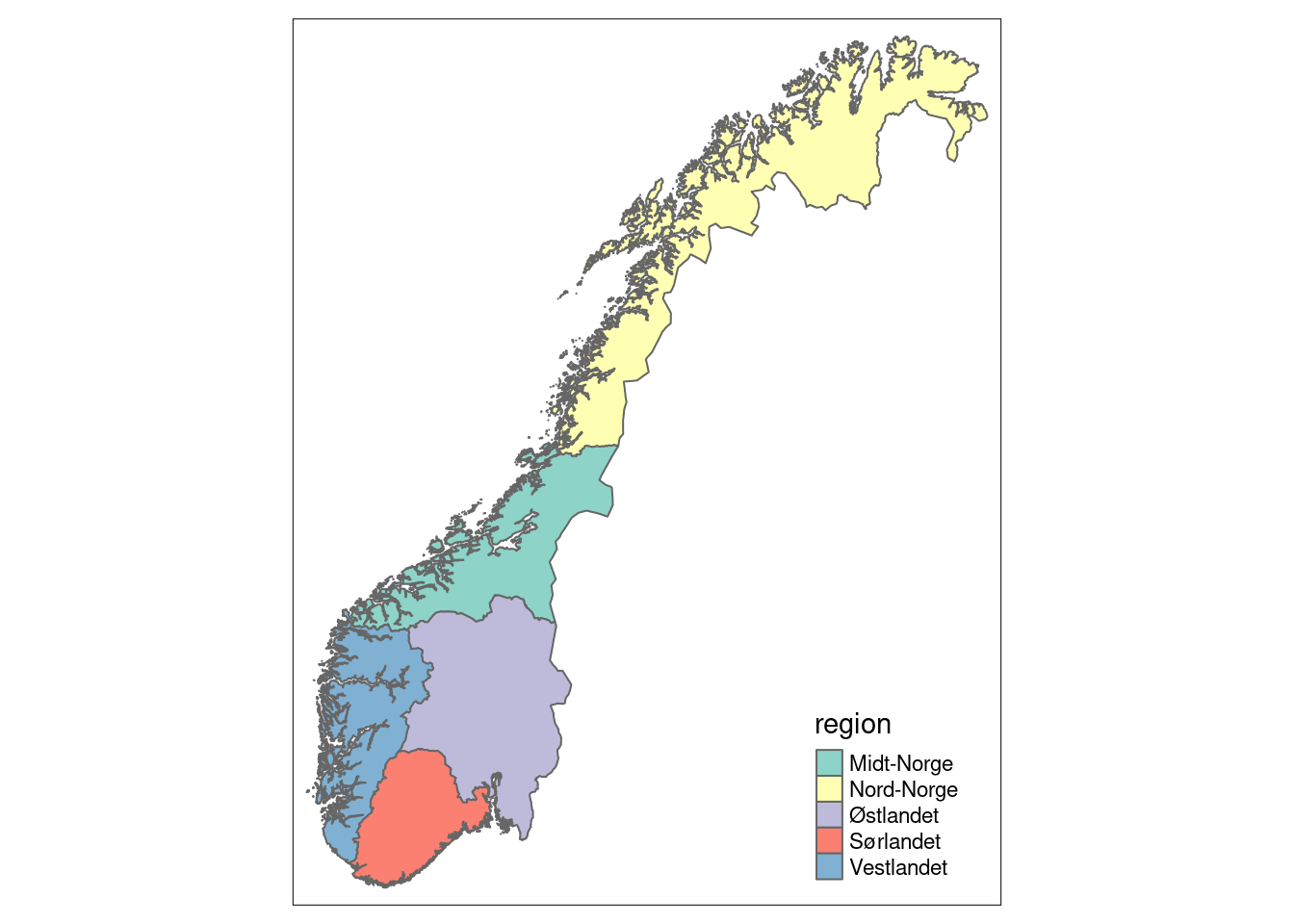
Figure 3.1: Five accounting areas (regions) in Norway.
4.8.2 Conceptual workflow
The general, the conceptual workflow is like this:
-
Collate variable data series
Import .nc files (loop though year 1961-1990) and subset to the correct attribute
Filter data by dates (optional) (
dplyr::filter). This means reading all 365 rasters into memory, and it is much quicker to filter out the correct rasters in the importing step above (see examples later in this chapter)Aggregate across time within a year (
stars::st_apply). This is the most time consuming operation in the workflow.Join all data into one data cube (
stars:c)
-
Calculate reference values
Aggregate (
st_apply)across reference years (dplyr::filter) to get median and sd valuesJoin with existing data cube (
stars:c)
-
Calculate indicator values
- Normalize climate variable at the individual grid cell level using the three reference values (
mutate(across()))
- Normalize climate variable at the individual grid cell level using the three reference values (
Mask by ecosystem type (This could also be done in step one, but it doesn’t speed things up to set some cells to NA)
-
Aggregate in space (to accounting areas) (zonal statistics)
Aggregate across 5 year time steps to smooth out random inter-annual variation and leave climate signal
Intersect with accounting area polygons
exactextrar::exact_extractand get mean/median and (spatial) sd. (Alternatively, get temporal sd at the grid cell level in the step above.)
Make trend figure and spatially aggregated maps
4.8.3 Step 1 - temporal aggregation within a year
path <- path <- ifelse(dir == "C:",
      "R:/",
      "/data/R/")

path2 <- paste0(path, "GeoSpatialData/Meteorology/Norway_SeNorge2018_v22.09/Original/rr_tm/")

myFiles <- list.files(path2, pattern=".nc$",full.names = T)
# The last file (the last year) is incomplete and don't include all julian dates that we select below, so I will not include it:
myFiles <- myFiles[-length(myFiles)]

real_temp_summer <- NULL

# set up parallel cluster using 10 cores
cl <- makeCluster(10L)

# Get julian days after defining months
temp <- stars::read_ncdf(paste(myFiles[1]), var="tg")
start_month_num <-  6
end_month_num <- 8

julian_start <- yday(st_get_dimension_values(temp, "time")[1] %m+%
                       months(+start_month_num))
julian_end <- yday(st_get_dimension_values(temp, "time")[1] %m+%
                     months(+end_month_num))
step <- julian_end-julian_start


for(i in 1:length(myFiles)){

  tic("init")
  temp <- stars::read_ncdf(paste(myFiles[i]), var="tg", proxy=F,
                           ncsub = cbind(start = c(1, 1, julian_start),
                              count = c(NA, NA, step)))
  year_temp <- year(st_get_dimension_values(temp, "time")[1])
  print(year_temp)
  lookup <- setNames("mean", paste0("v_", year_temp))
    # Perhaps leave out the v_ to get a numeric vector instead,
    # which is easier to subset
  st_crs(temp) <- 25833
  toc()

  tic("filter and st_apply")
  temp <- temp %>%
    #filter(time %within% myInterval) %>%
    st_apply(1:2, mean, CLUSTER = cl) %>%
    rename(all_of(lookup))
  toc()

  tic("c()")
  real_temp_summer <- c(temp, real_temp_summer)
  #rm(temp)
  toc()
}

tic("Merge")
real_temp_summer <- real_temp_summer %>%
  merge(name = "Year") %>%
  setNames("climate_variable")
toc()

stopCluster(cl)
This takes about 20 sec per file/year, or 22 min on total. That is not too bad. About 6000 rasters are read into memory. Here’s a test for the effect of splitting over more cores.
write_stars(real_temp_summer, "/data/P-Prosjekter2/41201785_okologisk_tilstand_2022_2023/data/climate_indicators/aggregated_climate_time_series/real_temp_summer.tiff")Note that GTiff automatically renames the third dimension band and also renames the attribute. I can rename them.
summer_median_temp <- real_temp_summer %>%
  st_set_dimensions(names = c("x", "y", "v_YEAR")) %>%
  setNames("temperature")
ggplot()+
  geom_stars(data = summer_median_temp[,,,c(1,11,66)], downsample = c(10, 10, 0)) +
  coord_equal() +
  theme_void() +
  scale_fill_viridis_c(option = "D") +
  scale_x_discrete(expand = c(0, 0)) +
  scale_y_discrete(expand = c(0, 0))+
  facet_wrap(~v_YEAR)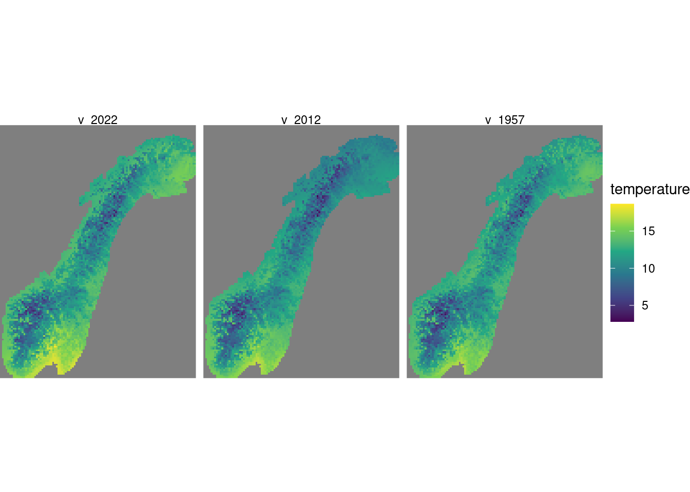
Figure 4.1: Showing three random slices of the year dimension.
4.8.4 Step 2 - calculate reference values
We need to first to define a reference period and then to subset our data summer_median_temp.
First we need to rename our dimension values and turn them back into dates.
new_dims <- as.Date(paste0(
  substr(st_get_dimension_values(summer_median_temp, "v_YEAR"), 3, 6), "-01-01"))
summer_median_temp_ref <- summer_median_temp %>%
  st_set_dimensions("v_YEAR", values = new_dims)
Then I can filter to leave only the reference period.
summer_median_temp_ref <- summer_median_temp_ref %>%
  filter(v_YEAR %within% interval("1961-01-01", "1990-12-31"))
st_get_dimension_values(summer_median_temp_ref, "v_YEAR")
#>  [1] "1990-01-01" "1989-01-01" "1988-01-01" "1987-01-01"
#>  [5] "1986-01-01" "1985-01-01" "1984-01-01" "1983-01-01"
#>  [9] "1982-01-01" "1981-01-01" "1980-01-01" "1979-01-01"
#> [13] "1978-01-01" "1977-01-01" "1976-01-01" "1975-01-01"
#> [17] "1974-01-01" "1973-01-01" "1972-01-01" "1971-01-01"
#> [21] "1970-01-01" "1969-01-01" "1968-01-01" "1967-01-01"
#> [25] "1966-01-01" "1965-01-01" "1964-01-01" "1963-01-01"
#> [29] "1962-01-01" "1961-01-01"
And then we calculate the median and sd like above
system.time({
cl <- makeCluster(10L)
summer_median_temp_ref <- summer_median_temp_ref %>%
  st_apply(c("x", "y"),
           FUN =  median_sd,
           CLUSTER = cl)
stopCluster(cl)
})| user | system | elapsed |
|---|---|---|
| 9.624 | 6.069 | 20.903 |
write_stars(summer_median_temp_ref, "/data/P-Prosjekter2/41201785_okologisk_tilstand_2022_2023/data/climate_indicators/aggregated_climate_time_series/summer_median_temp_ref.tiff")Pivot and turn dimension into attributes, and rename attributes:
summer_median_temp_ref_long <- summer_median_temp_ref %>%
  split("band") %>%
  setNames(c("reference_upper", "sd"))
tmap_arrange(
tm_shape(st_downsample(summer_median_temp_ref_long, 10))+
  tm_raster("reference_upper")
,
tm_shape(st_downsample(summer_median_temp_ref_long, 10))+
  tm_raster("sd",
            palette = "-viridis")
)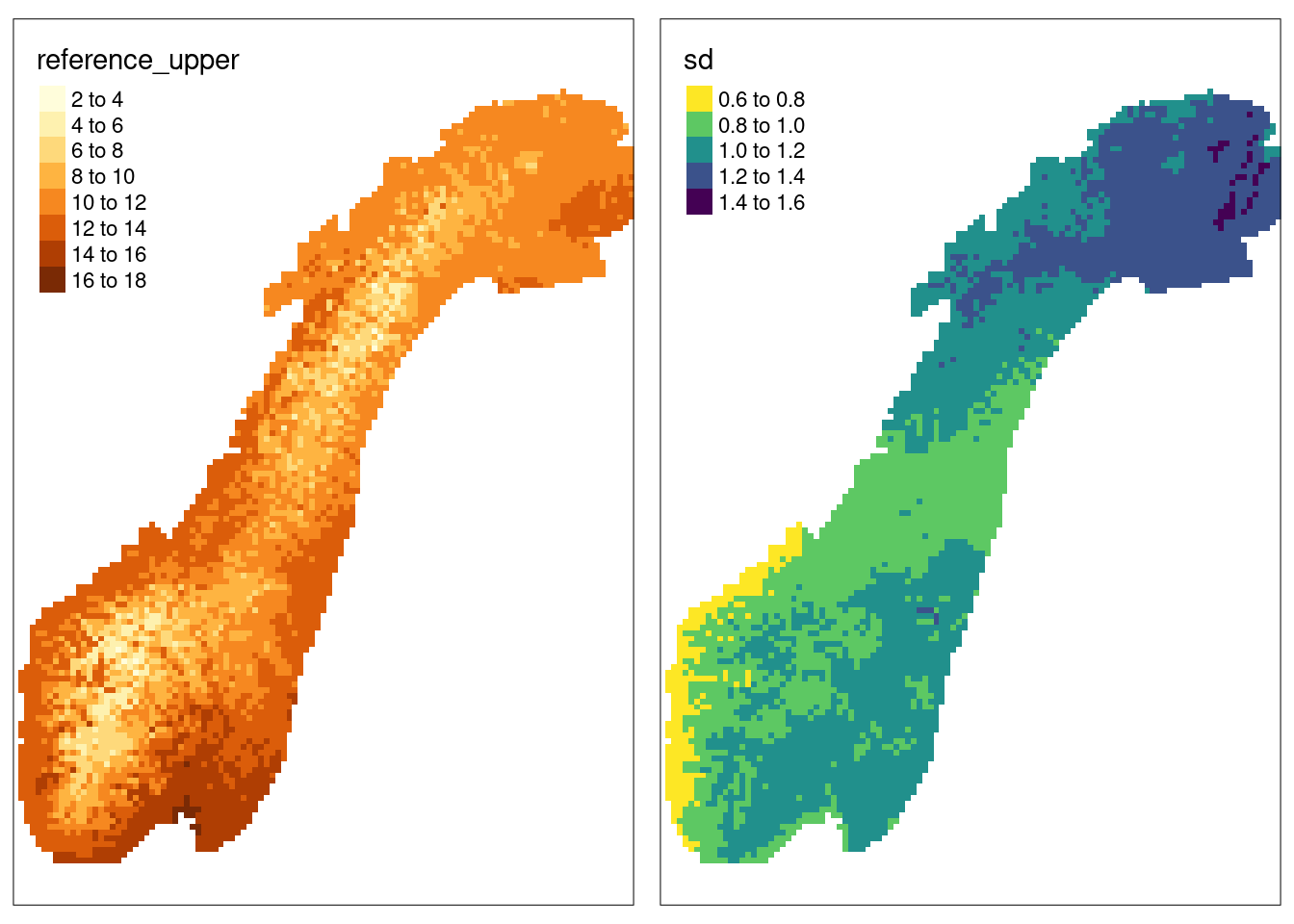
Figure 4.2: Showing the upper reference levels and the standard deviation from actual data of median summer temperatures.
I need to combine the variables and the ref values in one data cube
4.8.5 Step 3 - normalise variable
# select the columns to normalise
cols <- names(y_var)[!names(y_var) %in% c("reference_upper", "sd") ]
cols_new <- cols
names(cols_new) <- gsub("v_", "i_", cols)
# The break point scaling is actually not needed here, since
# having the lower ref value to be 5 sd implies that the threshold is
# 2 sd in a linear scaling.

system.time(
y_var_norm <- y_var %>%
  mutate(reference_low = reference_upper - 5*sd ) %>%
  mutate(reference_low2 = reference_upper + 5*sd ) %>%
  mutate(threshold_low = reference_upper -2*sd ) %>%
  mutate(threshold_high = reference_upper +2*sd ) %>%
  mutate(across(all_of(cols), ~
                  if_else(.x < reference_upper,
                  if_else(.x < threshold_low,
                                        (.x - reference_low) / (threshold_low - reference_low),
                                        (.x - threshold_low) / (reference_upper - threshold_low),
                                        ),
                  if_else(.x > threshold_high,
                                        (reference_low2 - .x) / (reference_low2 - threshold_high),
                                        (threshold_high - .x) / (threshold_high - reference_upper),
                                        )
                ))) %>%
  mutate(across(all_of(cols), ~ if_else(.x > 1, 1, .x))) %>%
  mutate(across(all_of(cols), ~ if_else(.x < 0, 0, .x))) %>%
  rename(all_of(cols_new)) %>%
  c(select(y_var, all_of(cols)))
)| user | system | elapsed |
|---|---|---|
| 14.803 | 2.717 | 17.512 |
gc()
saveRDS(y_var_norm, "/data/P-Prosjekter2/41201785_okologisk_tilstand_2022_2023/data/climate_indicators/aggregated_climate_time_series/summer_median_temp_normalised.RData")

# Tiff dont allow for multiple attributes:
#write_stars(y_var_norm, "/data/P-Prosjekter2/41201785_okologisk_tilstand_2022_2023/data/climate_indicators/aggregated_climate_time_series/summer_median_temp_normalised.tiff")
lims <- c(-5, 22)

ggarrange(
ggplot() +
  geom_stars(data = st_downsample(y_var_norm["v_1970"],10)) +
  coord_equal() +
  theme_void() +
  scale_fill_viridis_c(option = "D",
                       limits = lims) +
  scale_x_discrete(expand = c(0, 0)) +
  scale_y_discrete(expand = c(0, 0))
,
ggplot() +
  geom_stars(data = st_downsample(y_var_norm["reference_upper"], 10)) +
  coord_equal() +
  theme_void() +
  scale_fill_viridis_c(option = "D",
                       limits = lims) +
  scale_x_discrete(expand = c(0, 0)) +
  scale_y_discrete(expand = c(0, 0))
,
ggplot() +
  geom_stars(data = st_downsample(y_var_norm["reference_low"], 10)) +
  coord_equal() +
  theme_void() +
  scale_fill_viridis_c(option = "D",
                       limits = lims) +
  scale_x_discrete(expand = c(0, 0)) +
  scale_y_discrete(expand = c(0, 0))
,

ggplot() +
  geom_stars(data = st_downsample(y_var_norm["reference_low2"], 10)) +
  coord_equal() +
  theme_void() +
  scale_fill_viridis_c(option = "D",
                       limits = lims) +
  scale_x_discrete(expand = c(0, 0)) +
  scale_y_discrete(expand = c(0, 0))
,

ggplot() +
  geom_stars(data = st_downsample(y_var_norm["i_1970"],10)) +
  coord_equal() +
  theme_void() +
  scale_fill_viridis_c(option = "A",
                       limits = c(0, 1)) +
  scale_x_discrete(expand = c(0, 0)) +
  scale_y_discrete(expand = c(0, 0))
, ncol=2, nrow=3, align = "hv"
)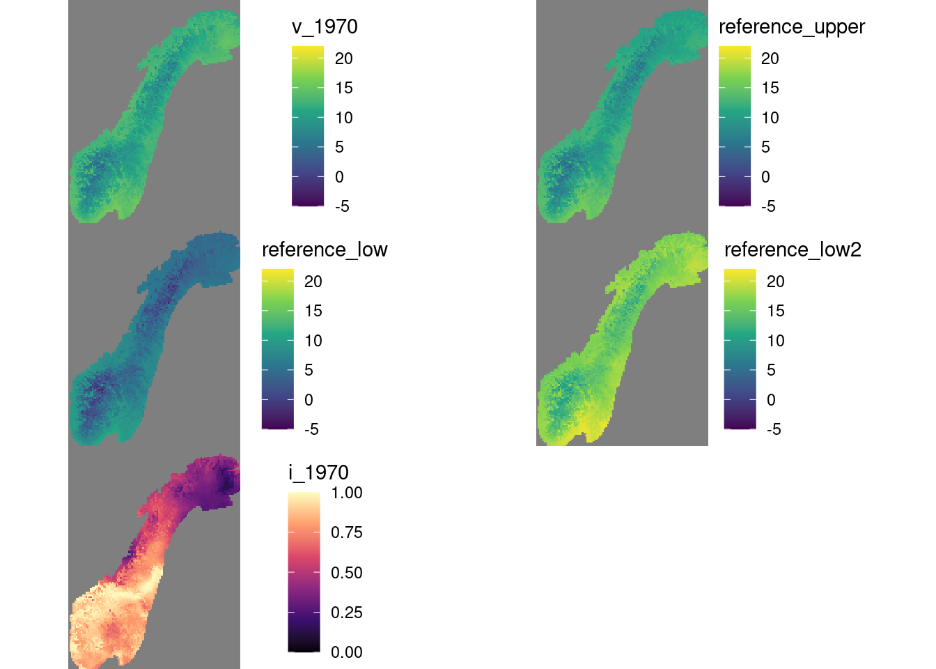
Figure 4.3: Example showing median summer tempretur in 1970, the upper and lwoer reference temperture, i.e. median and 5 SD units of the temperature between 1961-1990, and finally, the scaled indicator values.
The real indicator values should be means over 5 year periods. Calculating a running mean for all time steps is too time consuming. Therefore, the scaled, regional indicator values will be calculated for distinct time steps. The time series can perhaps still be presented with yearly resolution.
4.8.6 Step 4 - Mask with ecosystem delineation map
This step we simply ignore for now. It should be relatively easy to do, when we have the maps.
4.8.7 Step 5 - Make figures
To plot time series I first need to do a spatial aggregation.
system.time(
regional_means <- rast(y_var_norm) %>%
  exact_extract(reg, fun = 'mean', append_cols = "region", progress=T) %>%
  setNames(c("region", names(y_var_norm)))
  )
user; system; elapsed: 7.603; 3.071; 10.697
I could also get the sd like this, if I wanted to base the indicator uncertainty on a measure of spatial variation:
system.time(
regional_sd <- rast(y_var_norm) %>%
  exact_extract(reg, fun = 'stdev', append_cols = "region", progress=T) %>%
  setNames(c("region", names(y_var_norm)))
  )
user; system; elapsed: 7.420; 2.921; 10.355
Reshape and plot
div <- c("reference_upper",
         "reference_low",
         "reference_low2",
         "threshold_low",
         "threshold_high",
         "sd")

temp <- regional_means %>%
  as.data.frame() %>%
  select(region, div)

regional_means_long <- regional_means %>%
  as.data.frame() %>%
  select(!all_of(div)) %>%
  pivot_longer(!region) %>%
  separate(name, into=c("type", "year")) %>%
  pivot_wider(#id_cols = region,
              names_from = type)  %>%
  left_join(temp, by=join_by(region)) %>%
  mutate(diff = v-reference_upper) %>%
  mutate(threshold_low_centered = threshold_low-reference_upper) %>%
  mutate(threshold_high_centered = threshold_high-reference_upper)

#Adding the spatial sd
#(
#regional_means_long <- regional_sd %>%
#  select(!all_of(div)) %>%
#  pivot_longer(!region) %>%
#  separate(name, into=c("type", "year")) %>%
#  pivot_wider(names_from = type) %>%
#  rename(i_sd = i,
#         v_sd = v) %>%
#  left_join(regional_means_long, by=join_by(region, year))
#)
regOrder = c("Østlandet","Sørlandet","Vestlandet","Midt-Norge","Nord-Norge")

regional_means_long %>%
  mutate(col = if_else(diff>0, "1", "2")) %>%
  ggplot(aes(x = as.numeric(year),
           y = diff, fill = col))+
  geom_bar(stat="identity")+
  geom_hline(aes(yintercept = threshold_low_centered),
        linetype=2)+
  geom_hline(aes(yintercept = threshold_high_centered),
        linetype=2)+
  geom_segment(x = 1961, xend=1990,
               y = 0, yend = 0,
               linewidth=2)+
  scale_fill_hue(l=70, c=60)+
  theme_bw(base_size = 12)+
  ylab("Sommertemperatur\navvik fra 1961-1990")+
  xlab("")+
  guides(fill="none")+
  facet_wrap( .~ factor(region, levels = regOrder),
              ncol=3,
              scales = "free_y")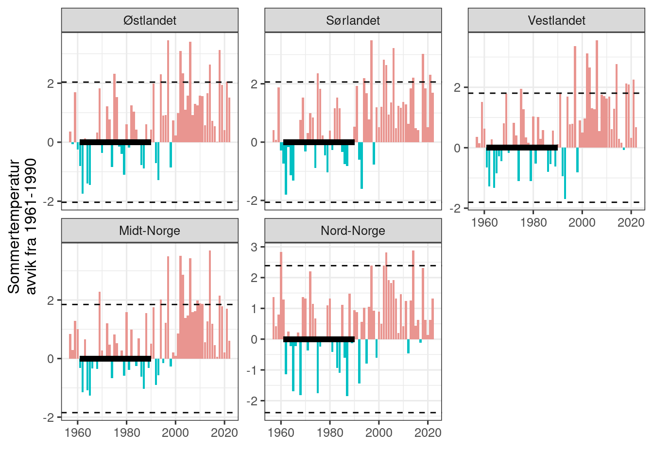
Figure 4.4: Times series for median summer temperature centered on the median value during the reference period. The reference period is indicated with a thick horizontal line. Dottet horisontal lines are 2 sd units for the reference period.
Then we can take the mean and sd over the last 5 years and add to a spatial representation.
(
i_aggregatedToPeriods <- regional_means_long %>%
  mutate(year = as.numeric(year)) %>%
  mutate(period = case_when(
    year %between% c(2018, 2022) ~ "2018-2022",
    year %between% c(2013, 2017) ~ "2013-2017",
    year %between% c(2008, 2012) ~ "2008-2012",
    year %between% c(2003, 2007) ~ "2003-2007",
    .default = "pre 2003"
  )) %>%
  mutate(period_rank = case_when(
   period == "2018-2022" ~ 5,
   period == "2013-2017" ~ 4,
   period == "2008-2012" ~ 3,
   period == "2003-2007" ~ 2,
    .default = 1
  )) %>%
  group_by(region, period, period_rank) %>%
  summarise(indicator = mean(i),
            sd = sd(i)
            # If I inluded a spatial measure for the uncertainty, here is how I would carry the errors:
            #spatial_sd = sqrt(sum(i_sd^2))/length(i_sd)
            )
)
#> `summarise()` has grouped output by 'region', 'period'. You
#> can override using the `.groups` argument.
#> # A tibble: 25 × 5
#> # Groups:   region, period [25]
#>    region     period    period_rank indicator     sd
#>    <chr>      <chr>           <dbl>     <dbl>  <dbl>
#>  1 Midt-Norge 2003-2007           2     0.427 0.139
#>  2 Midt-Norge 2008-2012           3     0.573 0.0992
#>  3 Midt-Norge 2013-2017           4     0.536 0.212
#>  4 Midt-Norge 2018-2022           5     0.607 0.179
#>  5 Midt-Norge pre 2003            1     0.642 0.182
#>  6 Nord-Norge 2003-2007           2     0.460 0.149
#>  7 Nord-Norge 2008-2012           3     0.675 0.0602
#>  8 Nord-Norge 2013-2017           4     0.641 0.127
#>  9 Nord-Norge 2018-2022           5     0.625 0.110
#> 10 Nord-Norge pre 2003            1     0.625 0.194
#> # ℹ 15 more rows
labs <- unique(i_aggregatedToPeriods$period[order(i_aggregatedToPeriods$period_rank)])

i_aggregatedToPeriods %>%
  ggplot(aes(x = period_rank,
             y = indicator,
             colour=region))+
  geom_line() +
  geom_point() +
  geom_errorbar(aes(ymin=indicator-sd,
                    ymax=indicator+sd),
                    width=.2,
                 position=position_dodge(0.2)) +
  theme_bw(base_size = 12)+
  scale_x_continuous(breaks = 1:5,
                     labels = labs)+
  labs(x = "", y = "indikatorverdi")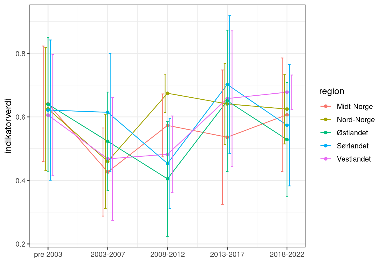
Figure 4.5: Scaled indicator values, aggregated over 5 year intervals. Errors represent temporal variation (standard errors) within regions and across 5 years.
Finally, I can add these values to the sp object with the accounting areas.
reg2 <- reg %>%
  left_join(i_aggregatedToPeriods[i_aggregatedToPeriods$period_rank==5,], by=join_by(region))
myCol <- "RdYlGn"
myCol2 <- "-RdYlGn"

tm_main <- tm_shape(reg2)+
  tm_polygons(col="indicator",
              title="Indikator:\nsommertemperatur",
    palette = myCol,
    style="fixed",
    breaks = seq(0,1,.2))

tm_inset <- tm_shape(reg2)+
  tm_polygons(col="sd",
              title="SD",
              palette = myCol2,
              style="cont")+
  tm_layout(legend.format = list(digits=2))

tmap_arrange(tm_main,
             tm_inset)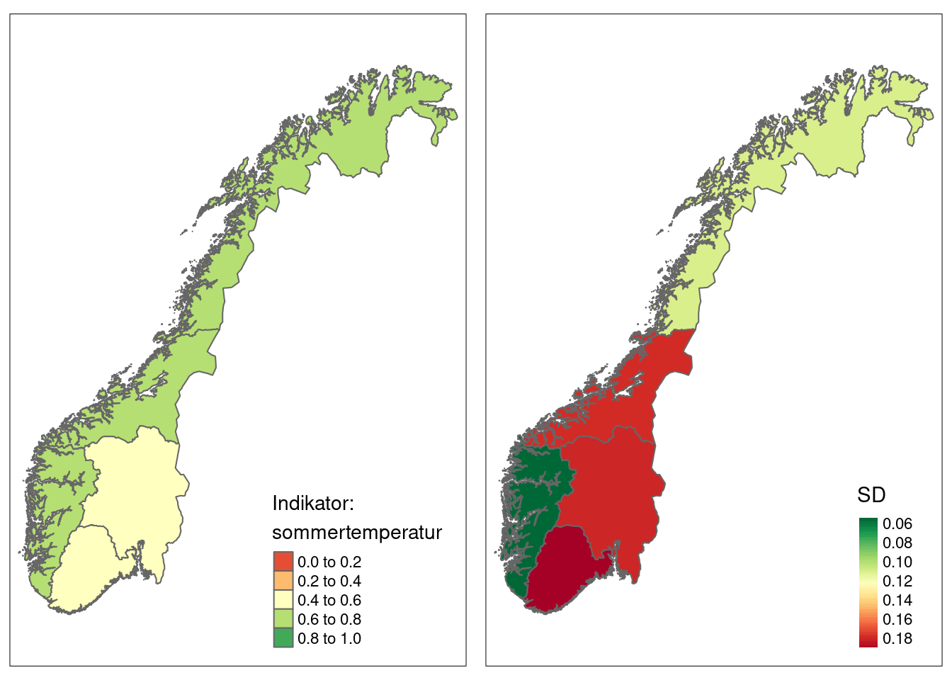
Figure 4.6: Summer tempreature indicator values for five accounting areas in Norway. SD is the spatial variation.