3 Anthropogenic disturbance to soils and vegetation (ADSV)
Author and date:
Anders L. Kolstad
September 2023
Norwegian indicator name: Slitasje
Ecosystem |
Økologisk egenskap |
ECT class |
|---|---|---|
Våtmark, Naturlig åpne områder under skoggrensa, Semi-naturlig mark |
Primærproduksjon (evt. Abiotiske fohold) |
Physical state characteristics |
3.1 Introduction
This indicator represent human caused damage or disturbance to soils and vegetation, typically from things like recreational activities and off-road vehicle traffic. The data come from a combination non-random field surveys and area-representative surveys. Disturbance to soils and vegetation is recorded in the various data sets are NiN variables 7SE and 7TK, or as the similar, but more fine-scaled variable, PRSL and PRTK. Effects from domestic animals are not included in the definition of these variables, and the upper reference value is therefore set to 0% disturbance.
The indicator is calculated separately for the three ecosystems, but all nature types associated with the same ecosystem are pooled and treated equally. This means we assume the nature types that are mapped and which we have data from are, when pooled, representative for the main ecosystem. This is less true for Naturally open ecosystems than it is for the other two. You can read more about that here.
Since the data is not sampled in a systematic or random way, we must take extra care not to over-extrapolate in space. We delineate homogeneous impact areas (HIA) based on four classes of increasing infrastructure, and we say that the field data is representative inside the HIA and region (five regions in Norway) where it was recorded. We then calculate an area weighted mean (and error) indicator value for each HIA and region combination, as long as there is more than 150 data points for a give combination of HIA and region.
Here is a general workflow for the calculation of the indicator.
Import Nature type data data set and ANO data set
Convert ANO points to polygons
For each polygon, extract the variable that has the lowest value (one-out all-out principle), e.g. Fig. 3.8. The four variables are 7TK, 7SE (both NiN2-variables) and PRTK and PRSL (both defined by the Norwegain Environmental Agency)
Combine data sets (nature types and ANO) but keep ecosystems separate.
Scale the
slitasjevariable based on reference values.Define homogeneous impact areas (HIA)
Aggregate and spread indicator value across HIAs and assessment regions
Confirm relationship between infrastructure index and indicator values to justify the extrapolation
TO DO: Prepare ecosystem delineation maps and us ethese to mask the extrapolated indicator maps
Spatial aggregation of indicator values and uncertainties to accounting areas
Export indicator maps and regional extrapolated maps
Note that besides the wetland map, we do not have ecosystem delineation maps to complete step 10 in the workflow.
| Variable | Name | Measurement scale | Description |
|---|---|---|---|
| 7TK | Spor etter ferdsel med tunge kjøretøy | A4b | Det som skal registreres er andelen (tenkte) småruter á 10 × 10 m (100 m2) innenfor en kartfigur som inneholder kjøretøyspor. |
| 7SE | Spor etter slitasje og slitasjebetinget erosjon | A4b | Det som skal registreres er antall (tenkte) småruter á 2 × 2 m (4 m2) som inneholder spor etter slitasje og slitasjebetinget erosjon (slitasjespor). |
| PRTK | Kjørespor | A8 | Same as 7TK, but with a finer measurement scale |
| PRSL | Slitasje | A8 | Same as 7SE, but with a finer measurement scale |
3.2 About the underlying data
The indicator uses a data set from a standardised field survey of nature types. You can read more about the preliminary analyses here. See also the official site of the Environment Agency. I also import a data set called ANO, which you can read about here
3.2.1 Representativity in time and space
The nature type mapping is not random and cannot be said to be area representative. The ANO data set however, is area representative. The data is from 2018 to present. The data from one field season usually becomes available early the following year.
3.2.2 Original units
The variables are recorded on a coarse four-step ordinal scale (Fig. 3.4) or eigth-step scale.
3.2.3 Temporal coverage
The data goes back to 2018. I therefore bulk all the data from 2018 to 2022 into one time step. I then use the mean date for the raw data, and define the variable as belonging to the year 2020 (read more here).
Regarding update frequency, the Nature type data set is not replicated, nor will it be in the future. We must therefore trust that the selection criteria for which areas to survey will not change drastically and systematically over time. For example, we are now surveying a lot in pressure areas, meaning lowland areas close to human population centers. If we in the future allocate more time to surveying wilderness areas, then the indicator becomes biased. On the other hand, ANO is replicated every 5 years.
3.2.4 Aditional comments about the dataset
For a run through of the nature type data set, see here.
3.3 Ecosystem characteristic
3.3.1 Norwegain standard
The indicator is tagged to the Økologisk egenskap called Primærproduksjon (Primary productivity). This is somewhat tentative, and perhaps abiotiske forhold is more suited. But the thought behind the choice is that ADSV affect the potential for primary productivity.
3.4 Collinearities with other indicators
ADSV is not thought to exhibit collinearity with any other indicator at the present.
3.5 Reference condition and values
3.5.1 Reference condition
The reference condition is one with minimal negative human impact. This is also true for semi-natural ecosystems. For example, in the reference condition, ADSV in semi-natural ecosystems is defined to be zero, even though at no point in time would this condition be realized.
3.5.2 Reference values, thresholds for defining good ecological condition, minimum and/or maximum values
For a further discussion on this topic, see GitHub issue 88.
Upper = 0%
Threshold = 10%
Lower = 100%
The upper reference value is 0% (no damage), and the lower reference value is 100%. Note that 100% damage does not mean that all the area must be scarred or damaged, but that all hypothetical quadrats around a point is affected (the variable is frequency-driven, and not amount-driven).
The threshold for good ecosystem condition is set to 10% damage. This is an expert judgement, and a rather weak one at that. In the future we should try to empirically validate the dose-response relationship, for example by comparing different variable scores with erosion rates or the potential for plant growth. This would need to be done specifically for each nature type.
The indicator value could be interpreted differently at the polygon vs landscape scale. At the polygon scale, 10% damage may seem like not that much, whilst at the landscape scale, 10% seems more serious.
Read about the normalisation here.
3.6 Uncertainties
Uncertainties/errors are estimated for aggregated indicator values by
bootstrapping individual indicator values 1000 times and calculating a
distribution of area weighted means. See the documentation for eaTools::ea_spread here.
This uncertainty is different from
the spatial variation which we could get more straight forward without
bootstrapping. When aggregating a second time,
from homogeneous impact areas to accounting areas, we assume a normal
distribution around the indicator values, with the already mentioned
errors, and sample n times from these and combine the resamples into an
a new, area weighted, distribution. The errors for the accounting areas
thus represents both the spatial variation, and the precision, of the
indicator values within the accounting areas.
3.7 References
Halvorsen, R. & Bratli, H. 2019. Dokumentasjon av NiN versjon 2.2 tilrettelagt for praktisk naturkartlegging: utvalgte variabler fra beskrivelsessystemet. – Natur i Norge, Artikkel 11 (versjon 2.2.0): 1–218 (Artsdatabanken, Trondheim; http://www.artsdatabanken.no.)
Miljødirektoratet 2022. Kartleggingsinstruks - kartlegging av terrestriske Naturtyper etter NiN2. URL: https://www.miljodirektoratet.no/publikasjoner/2022/januar/kartleggingsinstruks-kartlegging-av-terrestriske-naturtyper-etter-nin/
Miljødirektoratet 2023. Arealrepresnetativ Naturovervåking. Webpage. URL: https://www.miljodirektoratet.no/ansvarsomrader/overvaking-arealplanlegging/miljoovervaking/overvakingsprogrammer/natur-pa-land/arealrepresentativ-naturovervakning-ano/
3.8 Analyses
3.8.1 Data sets
3.8.1.1 Nature type mapping
This indicator uses the data set
Naturtyper etter Miljødirektoratets Instruks, which can be found
here.
See also here for a detailed description of the data set.
We also have a separate summary file where the nature types are manually mapped to the correct NiN-main typesand to the NiN variables that are recorded in each nature type. We can use this to find the nature types associated with the NiN main types that we are interested in.
naturetypes_summary_import <- readRDS("data/naturetypes/natureType_summary.rds")We are only interested in a mapping units that include our target variables.
myVars <- c('7TK', '7SE', 'PRTK', 'PRSL')
naturetypes_summary <- naturetypes_summary_import %>%
  rowwise() %>%
  mutate(keepers = sum(c_across(
    all_of(myVars))>0, na.rm=T)) %>%
  filter(keepers > 0) %>%
  select(Nature_type, NiN_mainType, Year)
This deleted 17 nature types and left us with these:
DT::datatable(naturetypes_summary)Importing and sub-setting the main data file, fix duplicate hovedøkosystem, calculate area, split one column in two, make numeric, and select target variables:
naturetypes <- sf::st_read(dsn = path) %>%
  filter(naturtype %in% naturetypes_summary$Nature_type) %>%
  mutate(hovedøkosystem = recode(hovedøkosystem,
                                 "naturligÅpneOmråderUnderSkoggrensa" = "naturligÅpneOmråderILavlandet"),
         area = st_area(.)) %>%
  separate_rows(ninBeskrivelsesvariable, sep=",") %>%
  separate(col = ninBeskrivelsesvariable,
           into = c("NiN_variable_code", "NiN_variable_value"),
           sep = "_",
           remove=F) %>%
  mutate(NiN_variable_value = as.numeric(NiN_variable_value)) %>%
  filter(NiN_variable_code %in% myVars)
#> Reading layer `Naturtyper_nin_0000_norge' from data source
#>   `/data/R/GeoSpatialData/Habitats_biotopes/Norway_Miljodirektoratet_Naturtyper_nin/Original/Naturtyper_nin_0000_norge_25833_FILEGDB/Naturtyper_nin_0000_norge_25833_FILEGDB.gdb'
#>   using driver `OpenFileGDB'
#> Simple feature collection with 117427 features and 36 fields
#> Geometry type: MULTIPOLYGON
#> Dimension:     XY
#> Bounding box:  xmin: -74953.52 ymin: 6448986 xmax: 1075081 ymax: 7921284
#> Projected CRS: ETRS89 / UTM zone 33N
#> Warning: There was 1 warning in `stopifnot()`.
#> ℹ In argument: `NiN_variable_value =
#>   as.numeric(NiN_variable_value)`.
#> Caused by warning:
#> ! NAs introduced by coercion
ggplot(data = naturetypes, aes(x = naturtype, fill = hovedøkosystem))+
  geom_bar()+
  coord_flip()+
  theme_bw(base_size = 12)+
  theme(legend.position = "top",
        legend.title = element_blank(),
        legend.direction = "vertical")+
  #guides(fill = "none")+
  xlab("")+
  ylab("Number of localities")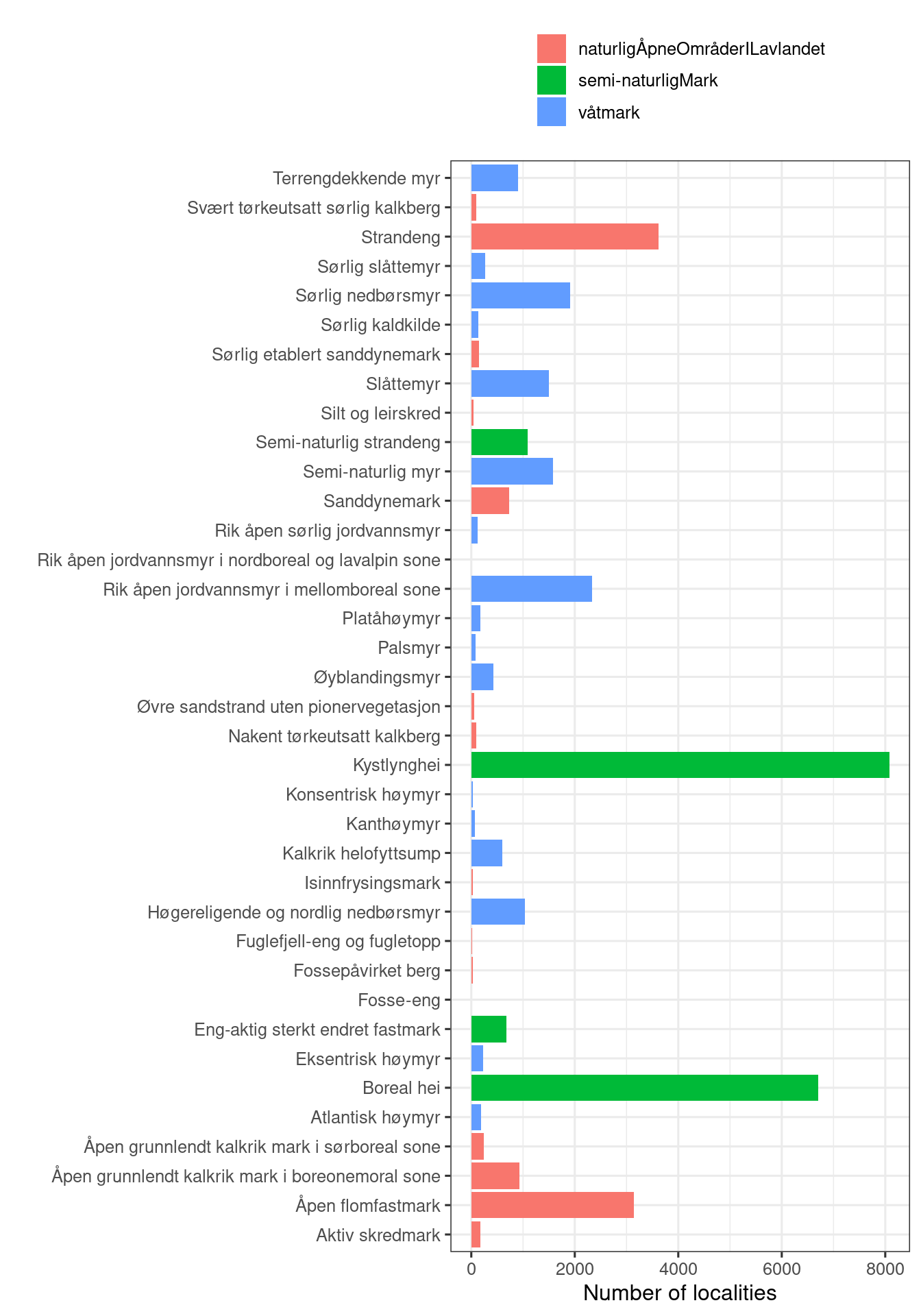
Figure 3.1: An overview of the naturetypes for which we will calculate the indicator. Colours refer to the main ecosystem affiliation.
Column names starting with a number is problematic, so adding a prefix
naturetypes$NiN_variable_code <- paste0("var_", naturetypes$NiN_variable_code)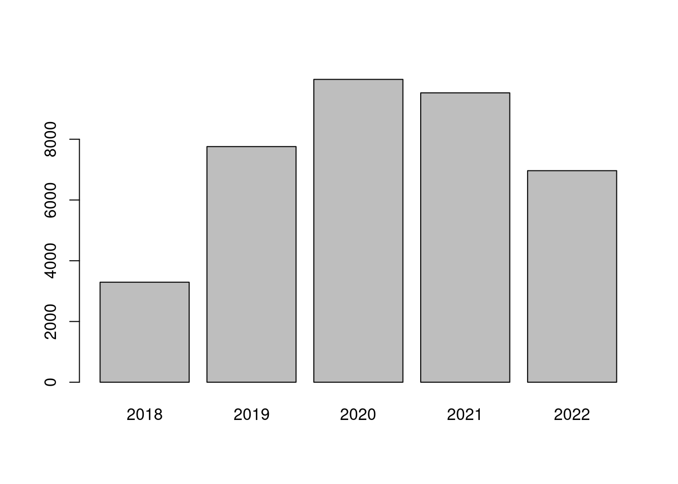
Figure 3.2: Distribution of data points over time.
Now I need to create a single row per locality with a new variable which is a product/function of the four variables “7SE”, “7TK”, “PRTK” and “PRSL”.
I initially baseed this indicator on whichever of the variables have the highest value (worst condition), but after some thought and discussion I now use an additive approach (adding the variable values togther). I first convert the ordinal scale to a continuous scale, using the median value of each ordinal step.
The variables use slightly different scales. PRSL and PRTK use this 8 step scale:
knitr::include_graphics("images/ninAR8.PNG")
Figure 3.3: Eight step condition scale
7TK and 7SE use a 4 step scale
knitr::include_graphics("images/ninAR4b.PNG")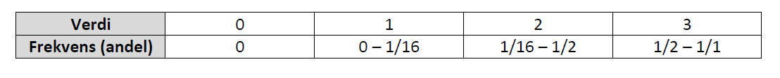
Figure 3.4: Four step condition scale
I here transfer these ordinal variables over to a continuous scale. The data is strongly right skewed, so simply taking the center value of each value range will not work.
naturetypes %>%
  ggplot()+
  theme_bw() +
  geom_histogram(aes(x = NiN_variable_value),
                 binwidth = 1) +
  facet_wrap(.~NiN_variable_code)
#> Warning: Removed 20 rows containing non-finite values
#> (`stat_bin()`).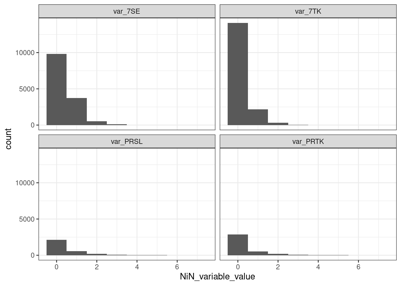
Figure 3.5: Histogram showing the distribution of the four variables used in this indicator.
The table below shows that, if I assume there is some ADSV and therefore exlude case with variable value <1, the median value for all the variables is 1. The most common % value for each range category should then be the lower limit of that category. For example, when the category is 1/2 - 1 then the % value is most likely 50%, and not 75% which is the center value for that value range. One issue is when the variable value is 1, because there the lower limit is the same as when the variable value is 0. Here I think I must manually assign it to something a bit higher than 0.
naturetypes %>%
  as.tibble() %>%
  filter(NiN_variable_value >0) %>%
  group_by(NiN_variable_code)%>%
  summarise(mean = mean(NiN_variable_value, na.rm=T),
            median = median(NiN_variable_value, na.rm=T))
#> Warning: `as.tibble()` was deprecated in tibble 2.0.0.
#> ℹ Please use `as_tibble()` instead.
#> ℹ The signature and semantics have changed, see
#>   `?as_tibble`.
#> This warning is displayed once every 8 hours.
#> Call `lifecycle::last_lifecycle_warnings()` to see where
#> this warning was generated.
#> # A tibble: 4 × 3
#>   NiN_variable_code  mean median
#>   <chr>             <dbl>  <dbl>
#> 1 var_7SE            1.18      1
#> 2 var_7TK            1.14      1
#> 3 var_PRSL           1.54      1
#> 4 var_PRTK           1.63      1
You can read more about this issue here.
naturetypes <- naturetypes %>%
  mutate(NiN_variable_value = case_when(
    NiN_variable_code %in% c("var_7TK", "var_7SE") ~
      case_match(NiN_variable_value,
             0 ~ 0,
             1 ~ mean(c(0, 1/16))*100,
             2 ~ 1/16*100,
             3 ~ 50),
    NiN_variable_code %in% c('var_PRTK', 'var_PRSL') ~
      case_match(NiN_variable_value,
             0 ~ 0,
             1 ~ 1.5,
             2 ~ 3,
             3 ~ 6.25,
             4 ~ 12.5,
             5 ~ 25,
             6 ~ 50,
             7 ~ 75)
    )
  )
This scaling of the variable implies that it very difficult to measure a location when it is in its most degraded form (100% disturbed), since the highest % value one can use is 75% for PRSL and PRTK and just 50% for the other two. This is a problem with the original data resolution. But I will compensate somewhat for this by using a non-linear transformation.
I will create a new data table where I calculate the new variable which I then paste back into the sf object.
naturetypes_wide <- pivot_wider(naturetypes,
                                names_from = "NiN_variable_code",
                                values_from = "NiN_variable_value",
                                id_cols = "identifikasjon_lokalId")
naturetypes_wide <- as.data.frame(naturetypes_wide)
head(naturetypes_wide, 10)
#>    identifikasjon_lokalId var_PRSL var_7TK var_7SE var_PRTK
#> 1         NINFP2210087853      0.0       0      NA       NA
#> 2         NINFP2210087857      0.0       0      NA       NA
#> 3         NINFP1910012022       NA      NA   0.000       NA
#> 4         NINFP1910005432      1.5      NA      NA       NA
#> 5         NINFP2210089748       NA       0   0.000       NA
#> 6         NINFP2210096062       NA      NA   0.000      0.0
#> 7         NINFP1910029434       NA      NA   3.125      1.5
#> 8         NINFP2010029112       NA       0   0.000       NA
#> 9         NINFP2010029325       NA       0   0.000       NA
#> 10        NINFP1910057556       NA      NA   0.000       NA
First I will combine 7TK and PRTK, and also 7SE and PRSL.
naturetypes_wide <- naturetypes_wide %>%
  mutate(TK = if_else(
    is.na(var_PRTK), var_7TK, var_PRTK),
    SE = if_else(
      is.na(var_PRSL), var_7SE, var_PRSL)
    )
SE has 10064 NA’s, and TK has 7007.
temp <- naturetypes_wide %>%
  group_by(SE) %>%
  summarise(sum = n())

ggplot(temp, aes(x = factor(SE),
                 y = sum))+
  geom_bar(stat="identity",
           fill="grey",
           colour = "black")+
  theme_bw(base_size = 12)+
  labs(x = "7SE or PRSL score",
       y = "Number of localities")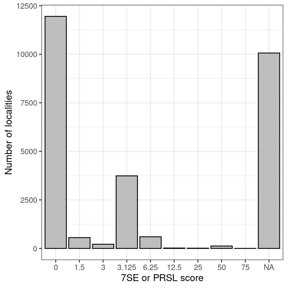
Figure 3.6: 7SE scores in the naturetype dataset
The NA fraction is quite big. These are localities with 7TK or PRTK recorded, but not 7SE or PRSL.
temp <- naturetypes_wide %>%
  group_by(TK) %>%
  summarise(sum = n())

ggplot(temp, aes(x = factor(TK),
                 y = sum))+
  geom_bar(stat="identity",
           fill="grey",
           colour = "black")+
  theme_bw(base_size = 12)+
  labs(x = "7TK og PRTK score",
       y = "Number of localities")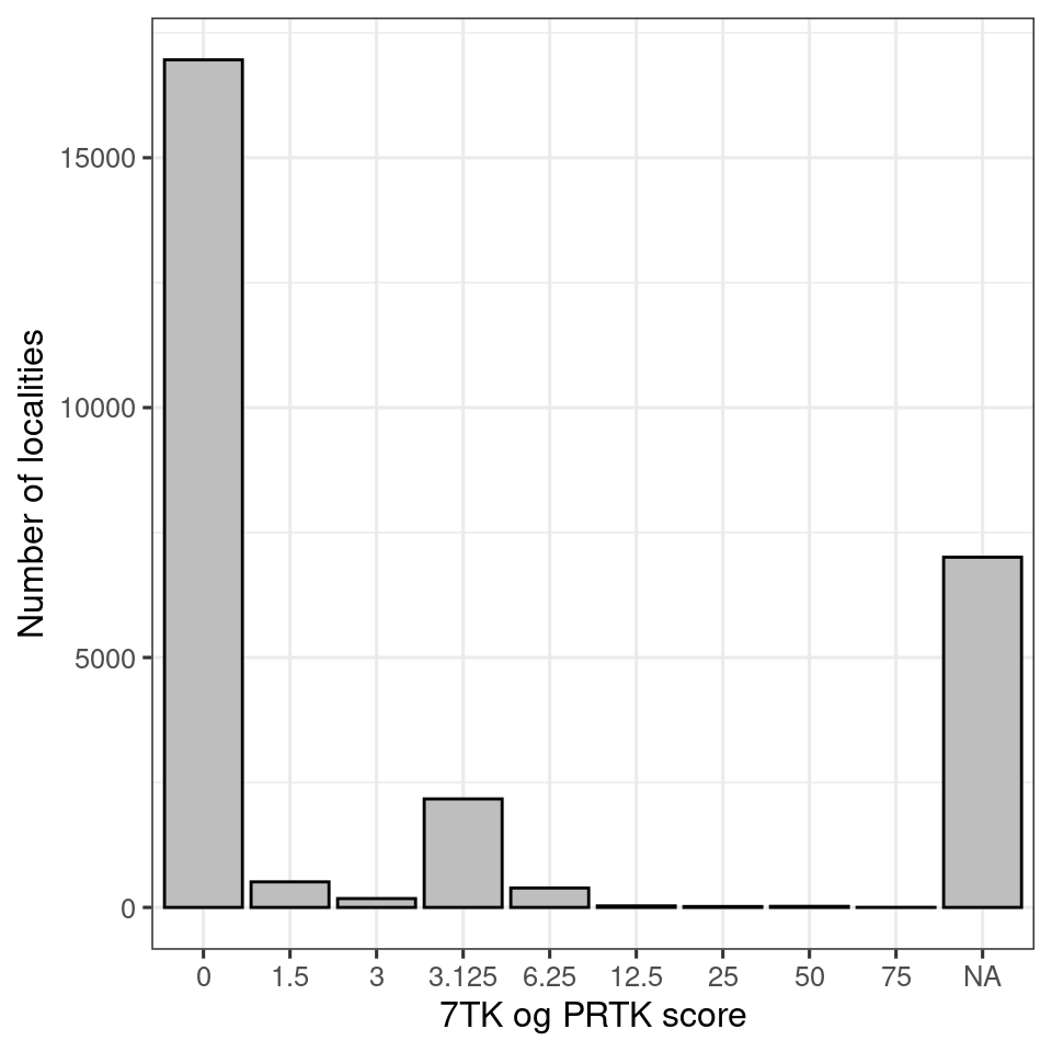
Figure 3.7: 7TK scores in the nature type dataset
Then I can add these two variables together into a composite variable called
slitasje
Chekhing for -Inf
nrow(naturetypes_wide[naturetypes_wide$slitasje<0,])
#> [1] 0
No issues with that.
temp <- naturetypes_wide %>%
  group_by(slitasje) %>%
  summarise(sum = n())

ggplot(temp, aes(x = slitasje,
                 y = sum))+
  geom_bar(stat="identity",
           fill="grey",
           colour = "black")+
  theme_bw(base_size = 12)+
  labs(x = "ADSV score converted to percentage",
       y = "Number of localities") +
  theme(axis.text.x = element_text(angle=90, vjust=0.5))+
  scale_x_continuous(
    labels = scales::label_number(accuracy = 1))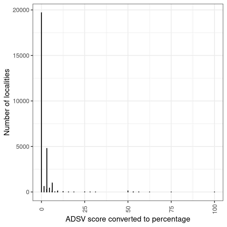
Figure 3.8: ADSV scores.
It appears most localities are in good condition. Note also that we theoretically can get >100% for the unscaled variable.
I would also like to know, when both TK and SE was recorded, which one is likely to be in the worst (or best) condition. I can do this by taking the difference.
diff <- naturetypes_wide$SE - naturetypes_wide$TK

diff <- ifelse(diff == 0, "TK and SE",
               ifelse(diff <0, "TK", "SE"))

diff_tbl <- as.data.frame(table(diff))

ggplot(diff_tbl, aes(x = diff, y = Freq))+
  geom_bar(stat = "identity",
           colour = "black",
           fill = "grey")+
  theme_bw(base_size = 12)+
  labs(x = "Variable indicating the worst state",
       y = "Number of localities")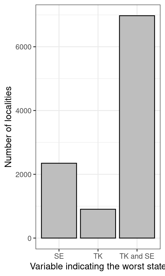
Figure 3.9: Counting the number of cases where TK or SE was in the worst condition for a given locality.
Looks like SE (= 7SE or PRSL) is more likely to be in a detrimental state.
Now I will copy these ADVS-values into the sf object.
3.8.1.2 GRUK
This variable is also recorded in
GRUK.
This is a stratified and intensive monitoring program for calcareous naturally open areas around the Oslo fjord.
The nature type data set I’m working on here includes some data from GRUK already
(presently only 2021 included). The full GRUK data set also contains a related variable:
% cover in 5m radii circles, which is much more detailed than the four variable we have looked at so far. This data is
not published. In any case it might be better to use the harmonized data set
in our case.
3.8.1.3 ANO
Arealrepresentativ Naturovervåking (ANO) consist of 1000 systematically placed locations each with 18 sample points. In each sample point a circle of 250 m2 is visualised, and the main ecosystem is recorded. Depending on the main ecosystem, certain NiN variables are also recorded. 7SE is recorded for våtmark (wetlands), but not semi-natural areas or naturally open areas. 7TK is recorded in wetlands and naturally open areas only.
| Variable | Våtmark | Naturlig åpne områder | Semi-naturlige områder |
|---|---|---|---|
| 7SE | X | - | - |
| 7TK | X | X | - |
It would be very nice to have 7SE recorded for naturally open areas. This variable is very relevant here.
I think I will only use wetlands here since my approach will be to the ‘worst value’ of the variable 7SE and 7TK (see below). I think not having 7SE for naturally open areas will underestimate the degree of degradation in these areas.
ANO could harmonise better with the Naturetype data set if it included 7SE and 7TK for Naturally open and Semi natural ecosystem.
ano <- sf::st_read(paste0(pData, "Naturovervaking_eksport.gdb"),
                   layer = "ANO_SurveyPoint") %>%
  dplyr::filter(hovedoekosystem_punkt == "vaatmark")
#> Reading layer `ANO_SurveyPoint' from data source
#>   `/data/P-Prosjekter2/41201785_okologisk_tilstand_2022_2023/data/Naturovervaking_eksport.gdb'
#>   using driver `OpenFileGDB'
#> Simple feature collection with 8974 features and 71 fields
#> Geometry type: POINT
#> Dimension:     XY
#> Bounding box:  xmin: -51950 ymin: 6467050 xmax: 1094950 ymax: 7923950
#> Projected CRS: ETRS89 / UTM zone 33N
table(ano$aar)
#>
#> 2019 2021
#>  130  558
This data set only contains data from year 2019 and 2021. We need to update this data set later. It is not clear why there is no data from 2020. This topic is maintained as a GitHub issue.
Each point/row here is 250 square meters. The data also contains information about how big a proportion of this area is made up of the dominant main ecosystem. However, there are 130 NA’s here, which is 19% of the data.
It appears the proportion of each circle that is made up of the dominant ecosystem was only recorded after year 2019. In fact, the main ecosystem was not recorded at all in 2019:
# Hard coding name change
#unique(ano$hovedtype_250m2)[3]
#ano$hovedtype_250m2[ano$hovedtype_250m2==unique(ano$hovedtype_250m2)[3]] <- "Aapen jordvassmyr"
table(ano$hovedtype_250m2, ano$aar)
#>
#>                              2019 2021
#>   Åpen jordvannsmyr             0  416
#>   Boreal hei                    0    1
#>   Fjellhei leside og tundra     0    3
#>   Grøftet torvmark              0    5
#>   Helofytt-ferskvannssump       0    3
#>   Kaldkilde                     0    2
#>   Myr- og sumpskogsmark         0   51
#>   Nedbørsmyr                    0   53
#>   Rasmark                       0    1
#>   Semi-naturlig myr             0    7
#>   Semi-naturlig våteng          0    2
#>   Skogsmark                     0    2
#>   Strandsumpskogsmark           0    2
#>   Våtsnøleie og snøleiekilde    0    6
I can remove the NA’s, and thus the 2019 data.
All of 2019 ANO data is excluded because of missing information
ano <- ano[!is.na(ano$andel_hovedoekosystem_punkt),]Let’s look at the variation in the recorded proportion of ecosystem cover
par(mar=c(5,6,4,2))
plot(ano$andel_hovedoekosystem_punkt[order(ano$andel_hovedoekosystem_punkt)],
     ylab="Percentage of the 250 m2 area\ncovered by the main ecosystem")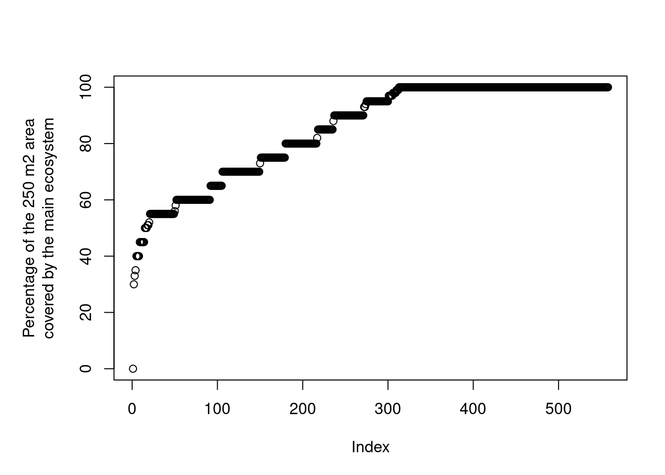
Figure 3.10: Distribution of the ANO variable andel_hovedoekosystem_punkt for wetland localities.
The zero in there is an obvious mistake.
ano <- ano[ano$andel_hovedoekosystem_punkt>20,]Here’s another plot of the distribution of the same variable:
ggplot(ano, aes(x = andel_hovedoekosystem_punkt))+
         geom_histogram(fill = "grey",
                        colour="black",
                        binwidth = 1)+
  theme_bw(base_size = 12)+
  xlab("Percentage cover of the Våtmark main ecosystem\n in the 250m2 circle")+
  scale_x_continuous(limits = c(0,101),
                     breaks = seq(0,100,10))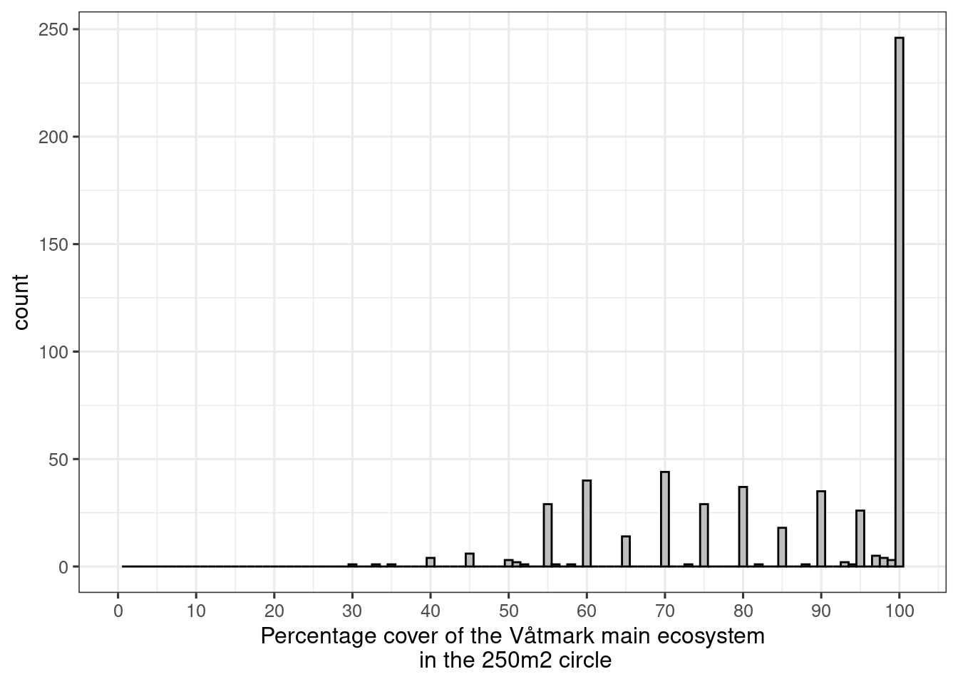
Figure 3.11: Percentage cover of the Våtmark main ecosystem in the 250m2 circle
We can see that people tend to record the variable in steps of 5%, and that most sample points are 100% belonging to the same main ecosystem.
We want to use area weighting in this indicator, so we can use this percentage cover data to calculate the area. Note that both data sets use m2 as area units.
ano$area <- (ano$andel_hovedoekosystem_punkt/100)*250Let’s now look at the distribution of the variables. First I need to separate the variable name from the values themselves. Now the data looks like this:
ano$bv_7se[1:6]
#> [1] "7SE_0" "7SE_0" "7SE_0" "7SE_0" "7SE_0" "7SE_0"
So I create a new variable prefixed var_:
ano$var_7SE <- as.numeric(sub(pattern = "7SE_",
                 replacement = "",
                 x = ano$bv_7se))
#> Warning: NAs introduced by coercion
The NA’s is the case of blank cells. The field app should not allow users leaving this field blank. I will need to remove these rows. There are fourteen cases:
ano <- ano[!is.na(ano$var_7SE),]Same with the other variable 7TK
ano$var_7TK <- as.numeric(sub(pattern = "7TK_",
                 replacement = "",
                 x = ano$bv_7tk))
No NA’s this time.
The ANO field app should not allow user to leave blank cells. This resulted in the exclusion of data.
par(mfrow=c(1,2))
barplot(table(ano$var_7TK), xlab="7TK scores")
barplot(table(ano$var_7SE), xlab="7SE scores")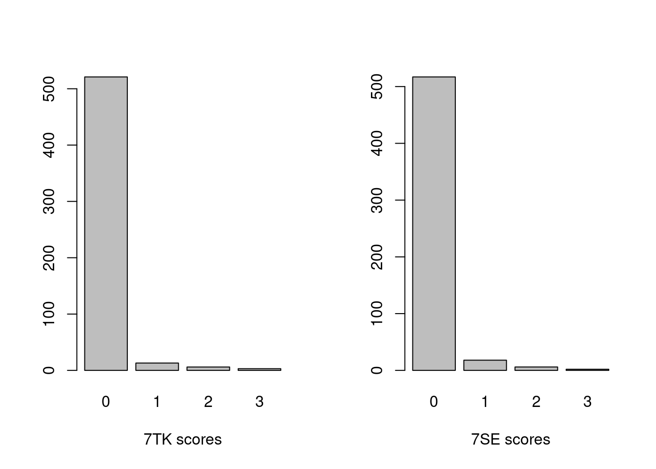
Figure 3.12: Distribution of 7TK and 7SE scores in the ANO data
The ANO sites seem to be in an even better condition than the localities in the naturtype data set.
Combining these two variables 7TK and 7SE into one, same as for the nature type data.
First I convert the range categories into percentages, like I did previously for the nature type data set.
ano <- ano %>%
  mutate(var_7TK = case_match(var_7TK,
             0 ~ 0,
             1 ~ mean(c(0, 1/16))*100,
             2 ~ 1/16*100,
             3 ~ 50)) %>%
  mutate(var_7SE = case_match(var_7SE,
             0 ~ 0,
             1 ~ mean(c(0, 1/16))*100,
             2 ~ 1/16*100,
             3 ~ 50))
temp <- as.data.frame(ano)
temp$slitasje <- apply(temp[,c("var_7TK", "var_7SE")], 1, sum, na.rm=T)
ano$slitasje <- temp$slitasje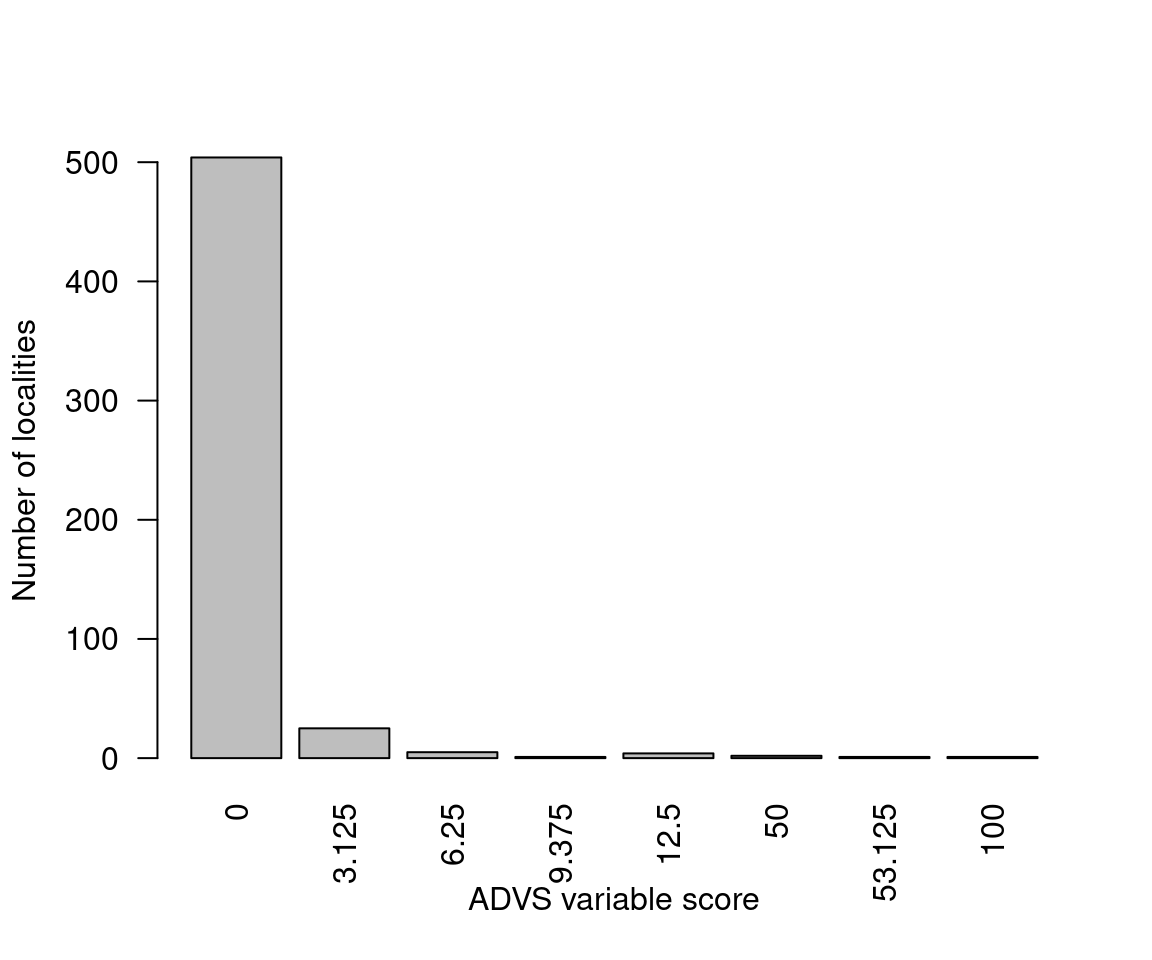
Figure 3.13: Distribution of slitasje scores in the ANO data
3.8.1.3.1 Combine Naturtype data and ANO
We need to combine the nature type data set with the ANO data set. I
will add a column origin to show where the data comes from. I will
also add a column with the main ecosystem.
ano$origin <- "ANO"
naturetypes$origin <- "Nature type mapping"
ano$hovedøkosystem <- "Våtmark"
ano$kartleggingsår <- ano$aar
Fix class
naturetypes$kartleggingsår <- as.numeric(naturetypes$kartleggingsår)
naturetypes$area <- units::drop_units(naturetypes$area)
I use dplyr::select to reduce the number of columns to keep things a
bit more tidy.
slitasje_data <- dplyr::bind_rows(select(ano,
                                  GlobalID,
                                  origin,
                                  kartleggingsår,
                                  hovedøkosystem,
                                  area,
                                  slitasje,
                                  SHAPE),
                           select(naturetypes,
                                  identifikasjon_lokalId,
                                  origin,
                                  hovedøkosystem,
                                  kartleggingsår,
                                  area,
                                  slitasje,
                                  SHAPE))

unique(st_geometry_type(slitasje_data))
#> [1] POINT        MULTIPOLYGON
#> 18 Levels: GEOMETRY POINT LINESTRING POLYGON ... TRIANGLE
3.8.1.3.1.1 Points to polygons
The ANO data is point data, and the nature type data is multipolygon. Because later we might want to save this as a shape file, we cannot have a mixed class type. I will therefore convert the points to polygons. I use the area column to calculate a radii that gives that area.
slitasje_data_points <- slitasje_data %>%
  mutate(g_type = st_geometry_type(.)) %>%
  filter(g_type =="POINT") %>%
  st_buffer(sqrt(slitasje_data$area/pi))
Checking now that the new polygons have the area corresponding to the proportion of the point that was part of the same main ecosystem:
slitasje_data_points$area2 <- st_area(slitasje_data_points)
plot(slitasje_data_points$area, slitasje_data_points$area2,
     xlab = "Target area",
     ylab = "Area of the new polygons")
abline(0,1)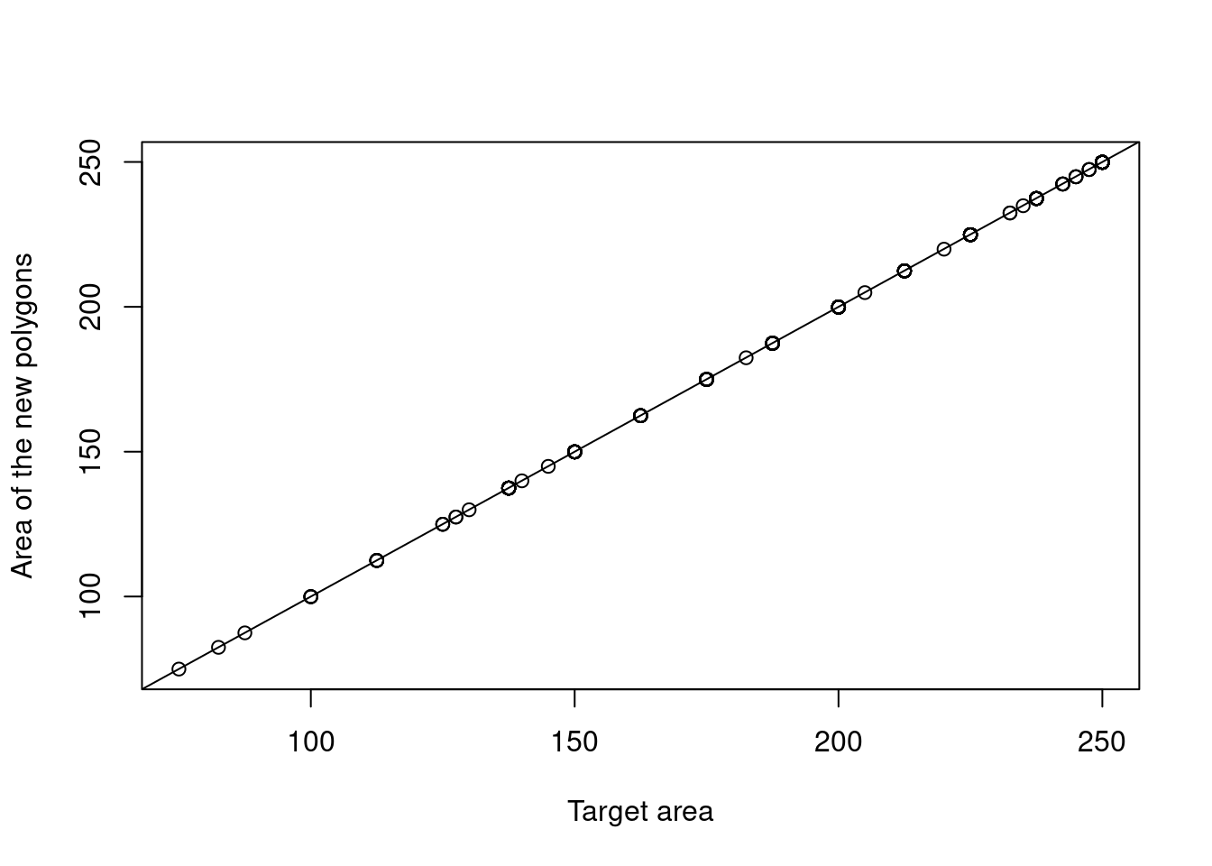
Figure 3.14: Checking that the area of the new polygons fall in line with the proportion of each point which is part of the main ecosystem.
The area calculation seems to have worked fine. Checking that the new data set contains only polygons.
slitasje_data_polygons <- slitasje_data %>%
  mutate(g_type = st_geometry_type(.)) %>%
  filter(g_type !="POINT")

slitasje_data <- bind_rows(slitasje_data_points, slitasje_data_polygons)

unique(st_geometry_type(slitasje_data))
#> [1] POLYGON      MULTIPOLYGON
#> 18 Levels: GEOMETRY POINT LINESTRING POLYGON ... TRIANGLE
Ok.
3.8.1.4 Distribution of ADVS scores
temp <- as.data.frame(table(slitasje_data$slitasje))
temp$Var1 <- as.numeric(as.character(temp$Var1))
ggplot(temp, aes(x = Var1,
                 y = Freq))+
  geom_bar(stat="identity",
           fill="grey",
           colour = "black")+
  theme_bw(base_size = 12)+
  labs(x = "ADVS score",
       y = "Number of localities")+
  scale_x_continuous(
    labels = scales::label_number(accuracy = 1))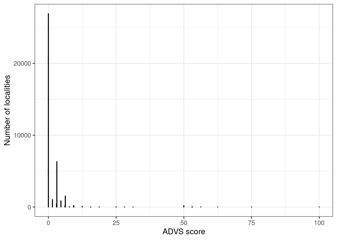
Figure 3.15: ADVS variable scores (ANO Naturetype data combined). The score for a locality equals the sum of the related variables 7TK, 7SE, PRSL and PRTK.
Let’s see the proportion of data points (not area) origination from each data set
temp <- as.data.frame(table(slitasje_data$origin))

ggplot(temp, aes(x = Var1,
                 y = Freq))+
  geom_bar(stat="identity",
           fill="grey",
           colour = "black")+
  theme_bw(base_size = 12)+
  labs(x = "Data origin",
       y = "Number of localities")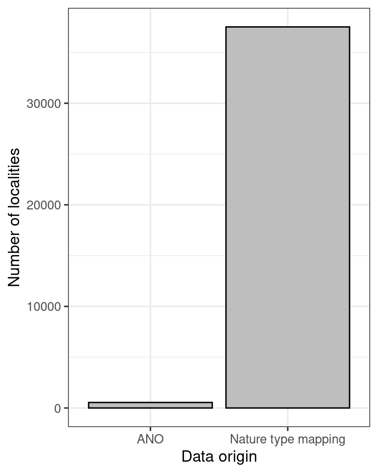
Figure 3.16: Barplot show the contribution (number of localities) of different data sets to the ADVS indicator.
So the ANO data is not very important here, but it can become more important in the future so good to have them included in the workflow.
3.8.1.5 Outline of Norway and regions
The GIS layers are used to crop out marine areas, and to define accounting areas, respectively.
outline <- sf::read_sf("data/outlineOfNorway_EPSG25833.shp")3.8.2 Scaled indicator values
I can scale the indicator for each polygon, or I can chose to aggregate them first. If the scaled value is representative and precise at the polygon level, then I could scale at that level. I think they are.
However, the combined surveyed area is a very small fraction of the total area of Norway, so that only producing indicator values for the mapped areas leaves the indicator without much value for regional assessments. When we do regional assessments and calculate regional indicator values, we cannot simply do an area weighting of the polygons in each region. This is because we don’t want to assume that the polygons are representative far outside of the mapped area. But perhaps we can assume them to be representative inside homogeneous ecological areas, or Homoegeneous Impact Areas (HIAs). That’s where the infrastructure index comes in. Here’s the plan:
normalise the indicators at the polygon level.
take a simplified infrastructure index (vector data set with HIAs) and extract the corresponding indicator values that intersect with a given HIA, and extrapolate the area weighted mean of those values to the entire HIA withing a given geographical region. Errors are calculated from bootstrapping.
Take the new area weighted indicator values for the HIAs and match them with ecosystem occurrences of the same HIA (possibly using randomly sampled points from the available ecosystem occurrences). The errors are the same as for the HIAs.
calculate an indicator value for a region (accounting area) by doing a weighted average based of the relative area of ecosystem occurrences. Errors should be carried somehow, perhaps via weighted resampling.
3.8.2.1 Scaled variable
I will use the same reference levels/values for all of Norway:
upper <- 0
lower <- 100
threshold <- 10
Also, the threshold value is set quite conservatively (I think), and should be discussed.
I need to do a little trick and reverse the upper and lower reference values for the normalisation to work. This is a bug which can be fixed inside eaTools.
eaTools::ea_normalise(data = slitasje_data,
                      vector = "slitasje",
                      upper_reference_level = lower,
                      lower_reference_level = upper,
                      break_point = threshold,
                      plot=T,
                      reverse = T
                      )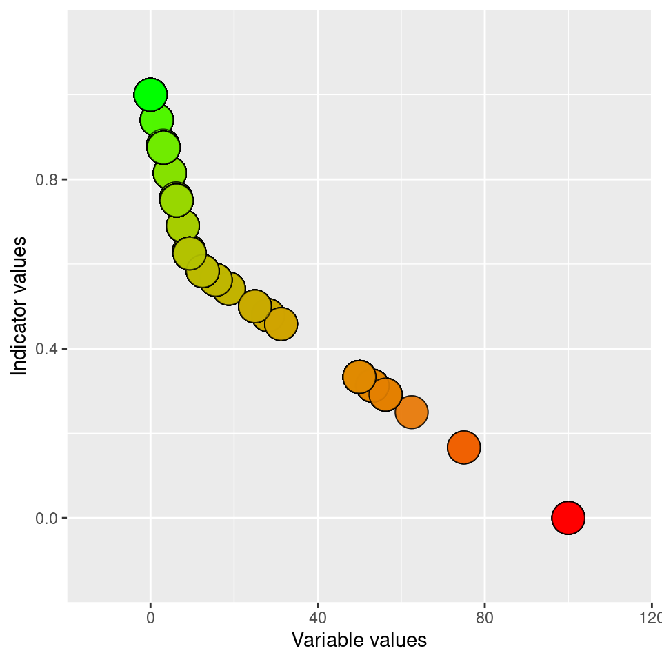
Figure 3.17: Performing a linear break-point type normalisation of the ADSV variable.
This normalisation seems reasonable to me. I can save it as indicator values. There is no point yet making this a time series, and I will assign all the indicator value to the average year of the data.
mean(slitasje_data$kartleggingsår)
#> [1] 2020.254
Assigning the indicator to year 2020.
slitasje_data$i_2020 <- eaTools::ea_normalise(data = slitasje_data,
                      vector = "slitasje",
                      upper_reference_level = lower,
                      lower_reference_level = upper,
                      break_point = threshold,
                      reverse = T
                      )
3.8.3 Homogeneous impact areas
I want to use the Homogeneous Impact Areas (HIA) to define smaller regions into which I can extrapolate the indicator values. This data is generated by discretizing the Norwegian Infrastructure Index. I refer to the ordinal values of the four HIA classes as their Human Impact Factor (HIF). This is just to keep the approach separate from the Norwegian Infrastructure Index.
I want to check that HIF is in fact a good predictor for slitasje.
I also want to split these four HIA classes based on their region. To do this I need the two layers to have the same CRS.
st_crs(HIA) == st_crs(regions)
#> [1] TRUE
Since the HIA map and the region map are completely overlapping (HIA was masked using the region map), we can get the intersections
HIA_regions <- eaTools::ea_homogeneous_area(HIA,
                             regions,
                             keep1 = "infrastructureIndex",
                             keep2 = "region")
saveRDS(HIA_regions, "P:/41201785_okologisk_tilstand_2022_2023/data/cache/HIA_regions.rds")
Create a new column by crossing region and HIF
HIA_regions <- HIA_regions %>%
  mutate(region_HIF = paste(region, infrastructureIndex))
3.8.3.1 Validate
I now have 20 unique areas (for each main ecosystem) that I will, given there is data, extrapolate indicator values over.
3.8.3.1.0.1 Subset ETs
I will subset the slitasje_data into the three ecosystems. Note that
only for open wetland do we have good ecosystem delineation maps to base
a spatial averaging on.
#Check spelling
#unique(slitasje_data$hovedøkosystem)

# Rename one level
slitasje_data <- slitasje_data %>%
  mutate(hovedøkosystem = recode(hovedøkosystem, "Våtmark" = "våtmark"))

#make valid
slitasje_data <- st_make_valid(slitasje_data)

#subset
wetlands <- slitasje_data[slitasje_data$hovedøkosystem == "våtmark",]
seminat <- slitasje_data[slitasje_data$hovedøkosystem == "semi-naturligMark",]
natOpen <- slitasje_data[slitasje_data$hovedøkosystem == "naturligÅpneOmråderILavlandet",]
Creating some summary statistics.
wetland_stats <- ea_spread(indicator_data = wetlands,
          indicator = i_2020,
          regions = HIA_regions,
          groups = region_HIF,
          summarise = TRUE)

seminat_stats <- ea_spread(indicator_data = seminat,
          indicator = i_2020,
          regions = HIA_regions,
          groups = region_HIF,
          summarise = TRUE)

natOpen_stats <- ea_spread(indicator_data = natOpen,
          indicator = i_2020,
          regions = HIA_regions,
          groups = region_HIF,
          summarise = TRUE)

wetland_stats <- wetland_stats %>%
  add_column(eco = "wetland")

seminat_stats <- seminat_stats %>%
  add_column(eco = "semi-natural")

natOpen_stats <- natOpen_stats %>%
  add_column(eco = "Naturally-open")

all_stats <- rbind(wetland_stats,
                   seminat_stats,
                   natOpen_stats)
all_stats <- all_stats %>%
  separate(region_HIF,
           into = c("region", "HIF"),
           sep = " ")

saveRDS(all_stats, "/data/P-Prosjekter2/41201785_okologisk_tilstand_2022_2023/data/cache/all_stats.rds")
temp_plot <- all_stats %>%
  mutate(HIF_NA = case_when(
    n > 150 ~ HIF
  ))

myColour_list <- unique(temp_plot$myColour)
names(myColour_list) <-   myColour_list

ggarrange(
ggplot(temp_plot, aes(x = region, y = n, group = HIF, fill = HIF_NA))+
  geom_bar(position = "dodge", stat = "identity", col="black")+
  theme_bw(base_size = 10)+
  scale_fill_brewer(palette="Oranges", na.translate=F)+
  theme(axis.text.x = element_text(angle = 90, vjust=0.5))+
  coord_flip()+
  labs(fill = "HIF")+
  geom_hline(yintercept=150)+
  facet_wrap(.~eco),
ggplot(temp_plot, aes(x = region, y = w_mean, group = HIF, fill = HIF_NA))+
  geom_bar(position = "dodge", stat = "identity", col="black")+
  theme_bw(base_size = 10)+
  scale_fill_brewer(palette="Oranges",  na.translate=F)+
  theme(axis.text.x = element_text(angle = 90, vjust=0.5))+
  coord_flip()+
  labs(fill = "HIF")+
  facet_wrap(.~eco),
ggplot(temp_plot, aes(x = region, y = sd, group = HIF, fill = HIF_NA))+
  geom_bar(position = "dodge", stat = "identity", col="black")+
  theme_bw(base_size = 10)+
  scale_fill_brewer(palette="Oranges",  na.translate=F)+
  theme(axis.text.x = element_text(angle = 90, vjust=0.5))+
  coord_flip()+
  labs(fill = "HIF")+
  facet_wrap(.~eco),
ncol = 1)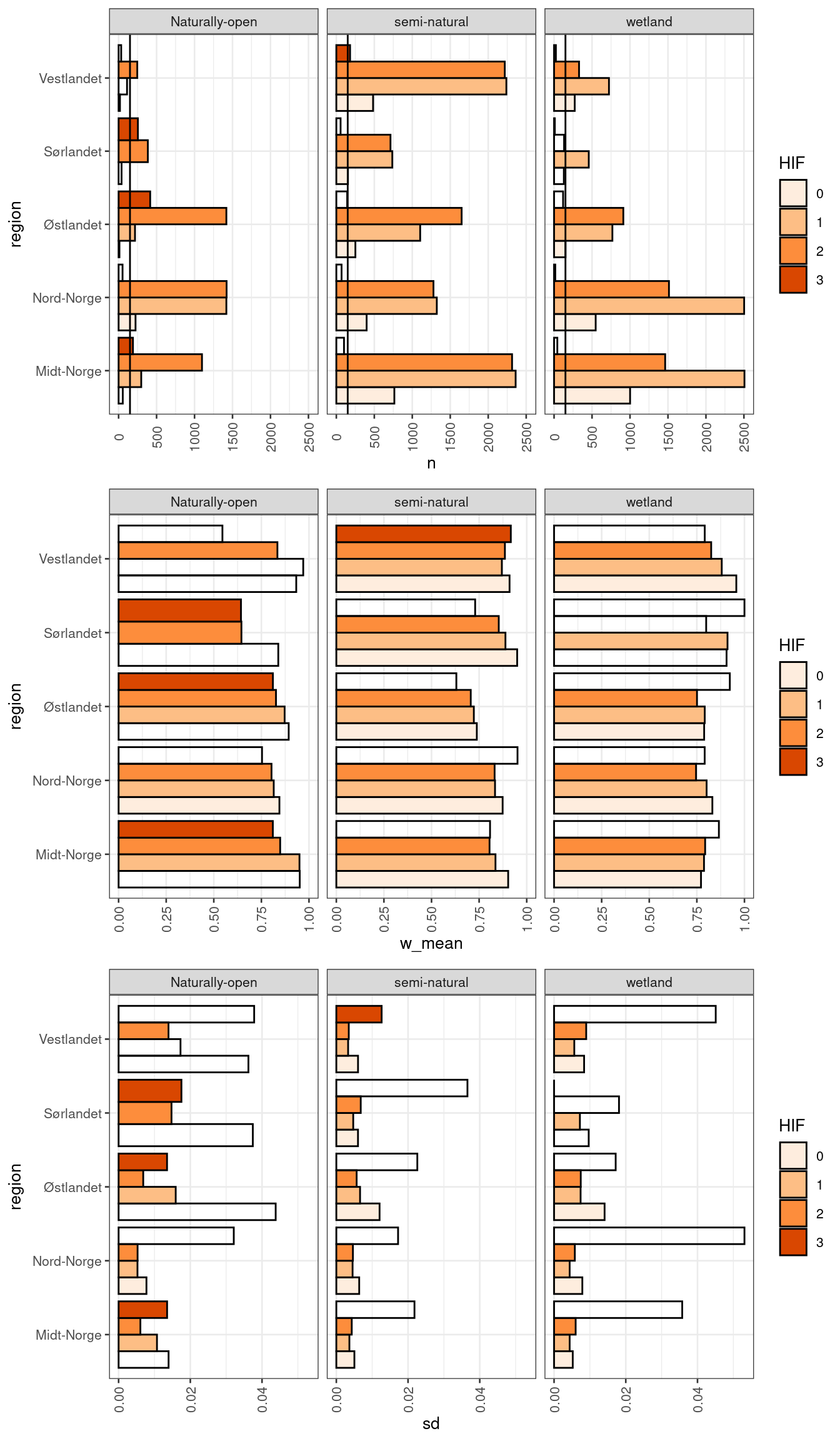
Figure 3.18: Barplot showing the number of data points, the area weighted scaled indicator values and the sd for the ADSV indicator. Transparent bars represents categories with less than 150 data points, indicated by the vertical line in the top row of panes.
In the figure above, colors refer to Human Impact Factor (amount or frequency of infrastructure) and NA means that there are less than 150 data points which we set as a threshold for evaluating the indicator values.
In the top row we see that the sample size (number of polygons) varies between ecosystems. For naturally open ecosystems many polygons are from high infrastructure areas, not surprisingly, and there are few points for the lowest impact class (zero such polygons in Sørlandet for example). We may therefore not be able to extrapolate indicator values for Naturally open areas in in Sørlandet with low levels of infrastructure.
In semi-natural areas and wetlands, we have very little data from HIF class 3.
We can also from the middle row see the association between the indicator values (area weighted means) and the modified infrastructure index (HIF). We should then not put any weight on the bars were there is little data (transparent bars). Then we se the general pattern that the indicator value decreases with increasing HIF. But there are exceptions, like for Semi-natural areas in Vestlandet.
Let us look at the indicator to pressure relationship across all ecosystems.
temp_plot %>%
  filter(!is.na(HIF_NA)) %>%
  ggplot(aes(x = HIF_NA, y = w_mean))+
  geom_point(size=2, position = position_dodge2(.1))+
  geom_violin(alpha=0)+
  theme_bw()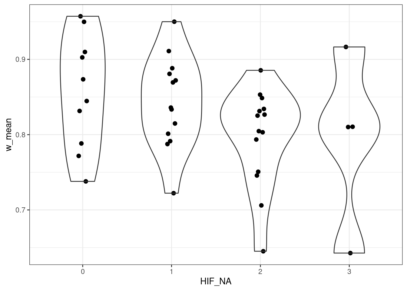
Figure 3.19: Indicator to pressure relationship across all ecosystems.
The pattern is not perfect, and there is quite some noise. But this is perhaps also expected.
Let us look at the effect of sample size on the indicator uncertainty.
temp_plot %>%
  ggplot(aes(x = n, y = sd))+
  geom_point(size=2, position = position_dodge2(.1))+
  theme_bw()+
    facet_wrap(.~eco)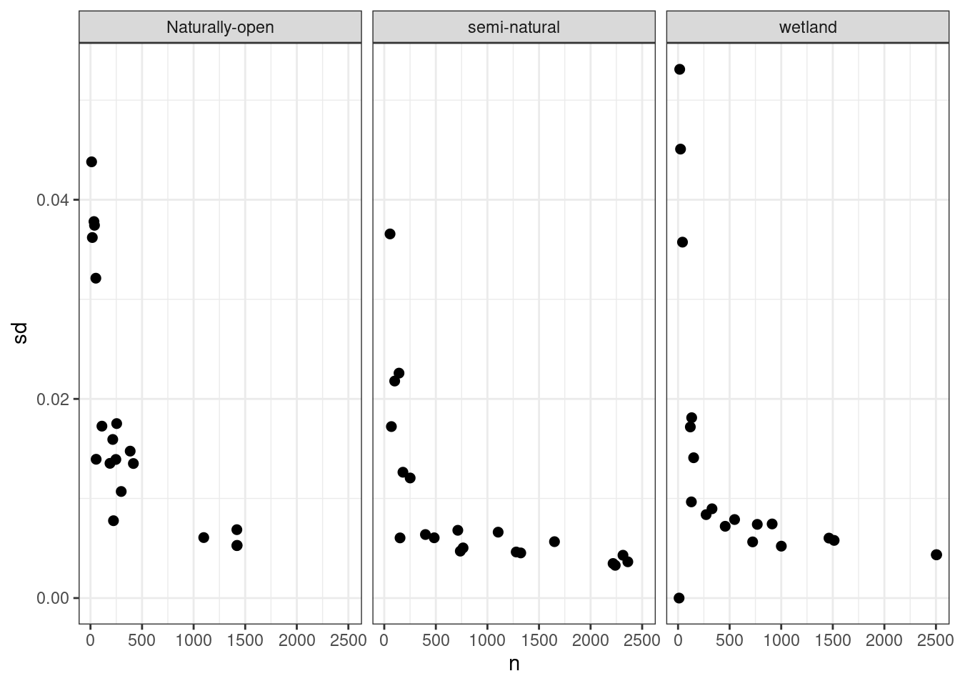
Figure 3.20: Smaple size against indicator uncertainty.
This shows that the uncertainty is inflated with sample sizes less than about 300-500.
DT::datatable(all_stats)Figure 3.21: Summary statistics for the slitasje indicator.
In addition to looking at the area weighted means and its relationship with the pressure indicator (HIF), we can do the same at the polygon level. Because the indicator is pseudo-continuous, boxplots for example become useless, so I will present a relative frequency plot.
corrCheck <- st_intersection(slitasje_data, HIA_regions)
saveRDS(corrCheck, "/data/P-Prosjekter2/41201785_okologisk_tilstand_2022_2023/data/cache/corrCheck.rds")
ggplot(corrCheck, aes(x = factor(infrastructureIndex), fill = factor(round(i_2020,2))))+
  geom_bar(position="fill")+
  theme_bw(base_size = 12)+
  guides(fill = guide_legend("Scaled indicator values"))+
  ylab("Fraction of data points")+
  xlab("HIF")+
  scale_fill_brewer(palette = "RdYlGn")+
  facet_grid(hovedøkosystem~region)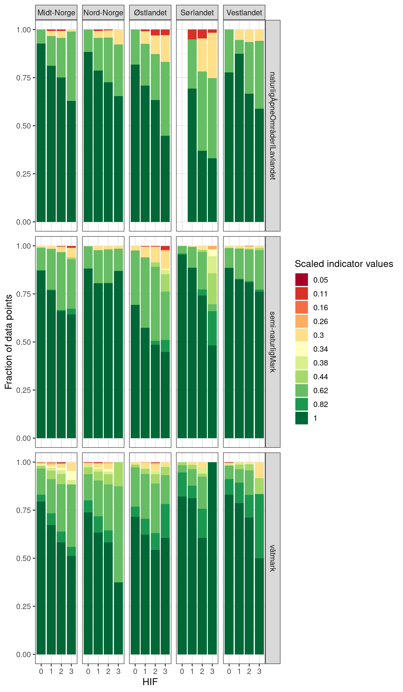
Figure 3.22: Relative frequency plot (conditioned on region and main ecosystem) showing the distribution of polygons with different scaled indicator values for the indicator named Anthropogenic disturbance to soils and vegetation.
The figure above I think supports the indicator-pressure relationship and justifies using the HIA+region intersections as local reference areas. Especially when down-weighting the importance of those groups/categories that have very little data.
3.8.3.2 Looking at the HIA
Here is a view of the data zooming in on Trondheim
myBB <- st_bbox(c(xmin=260520.12, xmax = 278587.56,
                ymin = 7032142.5, ymax = 7045245.27),
                crs = st_crs(HIA_regions))
Cropping the raster to the bbox
HIA_trd <- sf::st_crop(HIA_regions, myBB)
#> Warning: attribute variables are assumed to be spatially
#> constant throughout all geometries
Get map of major roads, for context
hw_utm <- readRDS("data/cache/highways_trondheim.rds")
(HIA_trd <- tm_shape(HIA_trd)+
  tm_polygons(col = "infrastructureIndex",
    title="Infrastructure index\n(modified 4-step scale)",
    palette = "-viridis",
    style="cat")+
  tm_layout(legend.outside = T)+
  tm_shape(hw_utm)+
  tm_lines(col="red")+
  tm_shape(outline)+
  tm_borders(col = "black", lwd=2))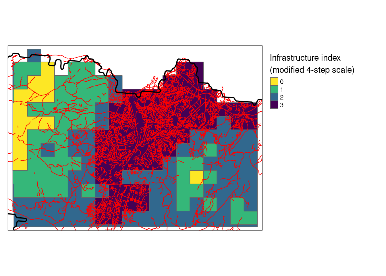
Figure 3.23: A closer look at the HIA designation over Trondheim
Let’s calculate the areas of these polygons and compare the HIF in the five regions.
HIA_regions$area <- sf::st_area(HIA_regions)
temp <- as.data.frame(HIA_regions) %>%
  group_by(region, infrastructureIndex) %>%
  summarise(area = mean(area))
#> `summarise()` has grouped output by 'region'. You can
#> override using the `.groups` argument.

ggplot(temp, aes(x = region, y = area, fill = factor(infrastructureIndex)))+
  geom_bar(position = "stack", stat = "identity")+
  guides(fill = guide_legend("HIF"))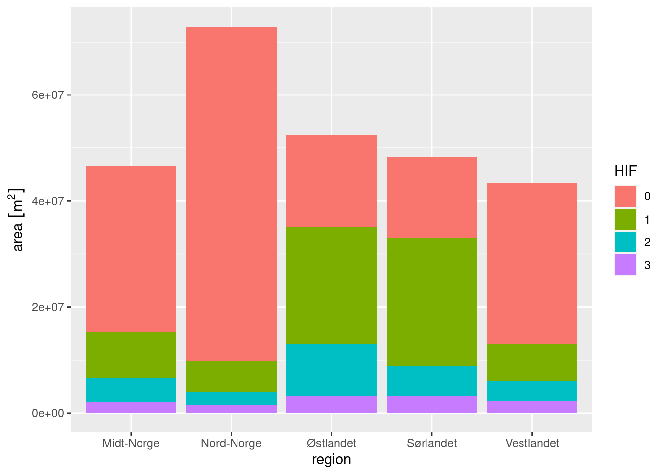
Figure 3.24: Stacked barplot showing the distribution of human impact factor across five regions in Norway.
The figure above shows that Nord-Norge for example, has a lot of relatively untouched areas, and that Østlandet has the highest proportion of impacted areas. This is expected.
3.8.4 Aggregate and spread (extrapolate)
I now want to find the mean indicator value for each HIA (i.e. to aggregate) and to spread these out spatially to the entire HIA within each region (i.e. to extrapolate).
I want to add a threshold so that we don’t end up over extrapolating based on too few data points. I have previousl used 150 data pionts, and I think that was about right.
wetlands_slitasje_extr <- ea_spread(indicator_data = wetlands,
                         indicator = i_2020,
                         regions = HIA_regions,
                         groups = region_HIF,
                         threshold = 150)

seminat_slitasje_extr <- ea_spread(indicator_data = seminat,
                         indicator = i_2020,
                         regions = HIA_regions,
                         groups = region_HIF,
                         threshold = 150)

natOpen_slitasje_extr <- ea_spread(indicator_data = natOpen,
                         indicator = i_2020,
                         regions = HIA_regions,
                         groups = region_HIF,
                         threshold = 150)
#saveRDS(wetlands_slitasje_extr, "/data/P-Prosjekter2/41201785_okologisk_tilstand_2022_2023/data/cache/wetlands_slitasje_extr.rds")
#saveRDS(seminat_slitasje_extr,  "/data/P-Prosjekter2/41201785_okologisk_tilstand_2022_2023/data/cache/seminat_slitasje_extr.rds")
#saveRDS(natOpen_slitasje_extr,  "/data/P-Prosjekter2/41201785_okologisk_tilstand_2022_2023/data/cache/natOpen_slitasje_extr.rds")
It’s easier to see what’s happening if we zoom in a bit. Lets get a boundary box around Trondheim.
myBB <- st_bbox(c(xmin=260520.12, xmax = 278587.56,
                ymin = 7032142.5, ymax = 7045245.27),
                crs = st_crs(wetlands_slitasje_extr))
Cropping the data to the bbox
wetlands_slitasje_extr_trd <- sf::st_crop(wetlands_slitasje_extr, myBB)
seminat_slitasje_extr_trd <- sf::st_crop(seminat_slitasje_extr, myBB)
natOpen_slitasje_extr_trd <- sf::st_crop(natOpen_slitasje_extr, myBB)
myCol <- "RdYlGn"
tmap_arrange(
tm_shape(wetlands_slitasje_extr_trd)+
  tm_polygons(col = "w_mean",
    title="Indicator value",
    palette = myCol,
    style="cont",
    breaks = c(0,1))+
  tm_layout(legend.outside = T)+
  tm_shape(hw_utm)+
  tm_lines(col="blue")+
  tm_layout(title = "Wetland"),

tm_shape(seminat_slitasje_extr_trd)+
  tm_polygons(col = "w_mean",
    title="Indicator value",
    palette = myCol,
    style="cont",
    breaks = c(0,1))+
  tm_layout(legend.outside = T)+
  tm_shape(hw_utm)+
  tm_lines(col="blue")+
  tm_layout(title = "Semi-natural areas"),

tm_shape(natOpen_slitasje_extr_trd)+
  tm_polygons(col = "w_mean",
    title="Indicator value",
    palette = myCol,
    style="cont",
    breaks = c(0,1))+
  tm_layout(legend.outside = T)+
  tm_shape(hw_utm)+
  tm_lines(col="blue")+
  tm_layout(title = "Naturally open areas"),
HIA_trd)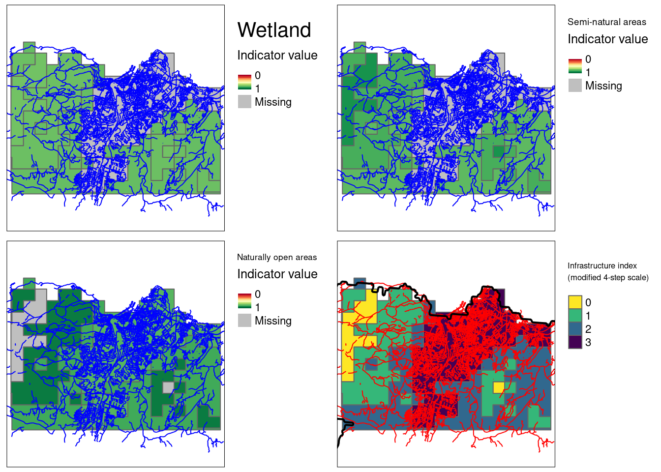
Figure 3.25: ADSV indicator extrapolated over Trondheim, with one map for each ecosystem. The map is not masked against ecosystem delineation maps, which make them easy to missinterpret.
Note that for wetland and semi-natural areas we did not extrapolate values for the most urban areas, and that for naturally open areas we did not extrapolate to the least affected areas. For the other regions we generally excluded more HIFs.
The maps above are easy to misunderstand, and they should therefor be communicated with caution. They should be considered as temporary files or as by-products.
The next step now is to
Prepare ecosystem delineation maps in EPSG25833 and perfectly aligned to a master grid
Rasterize the extrapolated indicator map, using the ET map as a template (see Fig. @ref(fig:#masking-example))
and mask it using the perfectly aligned ET map.
A faster way could be to:
Draw n random point samples from the ET map, and
extract indicator values at those points (from the extrapolated indicator map (a stars object)).
… but his will not provide spatially explicit indicator values for the entire ecosystem delineation.
3.8.5 Ecosystem map
See here.
3.8.6 Aggregate to region
We need to aggreate the ET occurence and their indicator values, to a
regional delineation. This functionality can be developed in eaTools,
but will in any case build around exactextratr::exact_extract().
To carry the errors, we can for example produce distributions for the indicator values for each ET occurrence (or groups of them) and resample the distributions with an area weighting.
3.9 Eksport files (final product)
According to the workflow specifications, I will export the indicator map at its highest resolution, for use in various web interfaces etc. For the finest resolution indicator map I will not include columns for uncertainty (because this will only be estimated at the aggregated level), or reference levels (because there is no spatial variation).
I can also export a map of the indicator where we extrapolate the indicator values to the homogeneous areas (e.g. Fig. 3.25 . This map should be interpreted with caution, since they appear as providing explicit indicator values for areas where there is no data. This map is mainly for aggregation purposes. I will mark this map with the prefix homogeneous-areas. I will also export this same map after masking it with the ET map, and this output must come with the same disclaimers.
Finally I will export a map of the five accounting areas with wall-to-wall indicator value and errors (e.g. Fig 4.6). This map can also contain data covering other ETs. Otherwise the maps would not we visually interpretative.
3.9.1 ADSV in wetlands
This is how I plan to export the final product.
# keep col names short and standardized
exp_wetland <- ...
exp_wetland_HIAextrapolated <- …exp_wetland_AAextrapolated <- …Write to file
st_write(exp_wetland, "indicators/indicatorMaps/slitasje/wetland_slitasje.shp",
         append = F)

st_write(exp_wetlandHIAextrapolated,
         "indicators/indicatorMaps/extrapolated_to_homogeneous_areas/slitasje/homogeneous_areas_wetland_slitasje.shp",
         append = F)

st_write(exp_wetland, "indicators/indicatorMaps/extrapolated_to_accounting_areas/slitasje/accounting_areas_wetland_slitasje.shp",
         append = F)