12 Connectivity
Norwegian name: Konnektivitet
Author and date:
Vegar Bakkestuen
November 2023
Ecosystem |
Økologisk egenskap |
ECT class |
|---|---|---|
Våtmark |
Landskapsøkologiske mønstre |
Landscape and seascape characteristics |
12.1 Introduction
Loss of natural habitat and changes in landscape patterns are central issues in biogeography and conservation biology. The loss of connectivity (connections or linkages) between suitable habitats affects individuals, populations, and communities through various ecosystem interactions. In landscape ecology, connectivity is essentially defined as “the degree to which the landscape facilitates or impedes movement between patches of resources or suitable habitats.” The concept of connectivity encompasses both structural connectivity, which involves the physical locations of suitable and unsuitable habitats or patches being analyzed, and functional connectivity, which focuses on the actual movement of individuals across suitable and unsuitable habitats and disturbance barriers. We have assessed that there is currently insufficient data available to start calculating functional connectivity on a national scale in relation to the assessment of ecological condition, as there is almost a total lack of relevant data for almost all species. Therefore, we have developed an index for structural connectivity based on physical interventions calculated using an infrastructure index (Erikstad et al. 2023) and a new wetland map for Norway (Bakkestuen et al. 2023, Bakkestuen et al. in prep).
Here a general workflow for the calculation of the indicator.
- You must load the necessary libraries for geospatial analysis.
- You must load the infrastructure index and wetland data.
- You define the buffer distance (500 meters).
- You must create a function (
calculateMeanDistance) to calculate the mean distance to infrastructure within a buffer around each wetland polygon. - Then you filter and keep only the homogeneous wetlands with more than 80% probability in the AI model for mire coverage.
- You have to apply the
calculateMinimumnDistancefunction to these selected wetlands, both with and without infrastructure. - You export the results as shapefiles for both scenarios.
- The scaled values for the “Connectivity” indicator are determined by comparing two scenarios: one that includes the presence of infrastructure and one that excludes infrastructure. The reference value is calculated as the ratio of the mean distances between myrpolygon areas in these two scenarios.
Currently step 8, and a subsequent step 9 (to aggregate scaled indicators to regions and simultaneously calculate errors) are not complete. Se this issuehttps://github.com/NINAnor/ecosystemCondition/issues/144.
It is also possible to create a time series for this indicator, but this is not yet done. See GitHub issue.
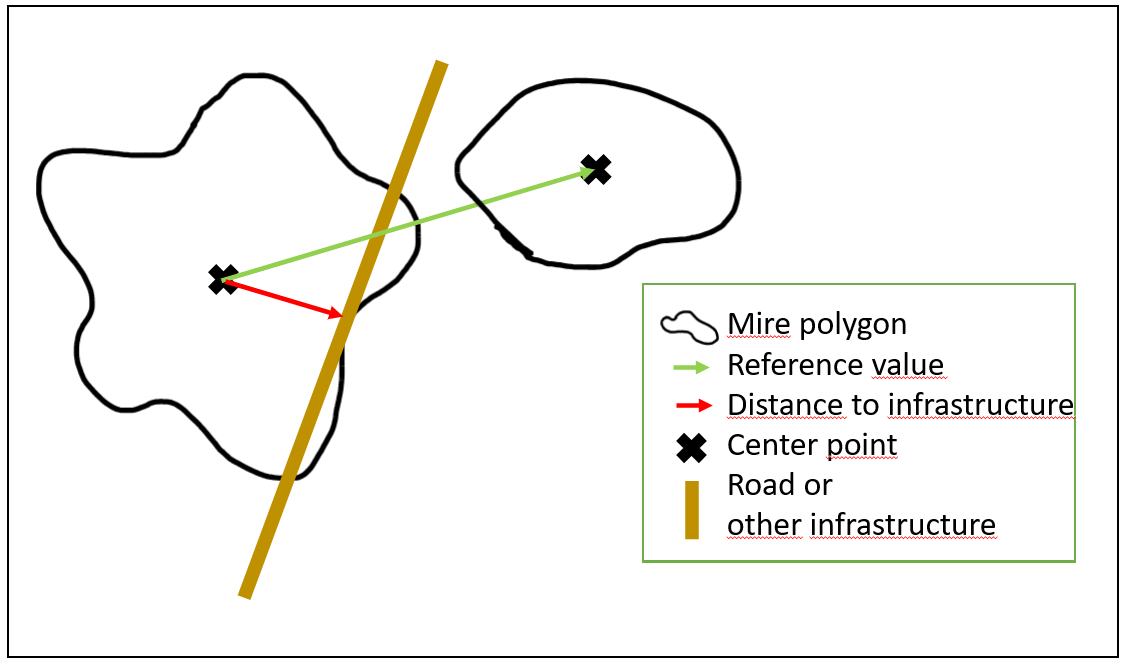
Figure 12.1: Conceptual model for the calculation of the conectivity indicator. Two distances are calculated: one from the centre point of one mire polygon to the closest neighbouring polygon (green arrow = the reference value), and one from the same centre point to the closest infrastructure (red arrow = area with infrastructure index value above 3). The scaled indicator is the ratio, or quotient, of the length of the red arrow divided by the length of the green arrow.
12.2 About the underlying data
The infrastructure index is one part of the connectivity index for wetlands. The infrastructure index was calculated for three time points: 2003, 2013, and 2023. This provides a temporal perspective for assessing changes over time. The data used included information on various types of infrastructure, such as roads and buildings. Additionally, a new wetland map for Norway has been developed. This map is based on Sentinel-2 and LiDAR data from the year 2020. The U-Net model, implemented through Google Earth Engine and TensorFlow, has been used for mapping wetlands in southern Norway. The model achieved a balanced accuracy rate of 90.9% when validated against ground-truth samples, significantly improving upon the accuracy rates achieved with manually digitized maps in Norway.
12.2.1 Representativity in time and space
The data for the infrastructure index covers the entire country and was collected for three time points over a 20-year period. This provides a broad and representative dataset for assessing changes in connectivity in Norwegian landscapes. The wetland mapping was conducted using data from the year 2020, making it representative for that specific time frame. However, the model used in the mapping process can be applied to other time frames if necessary.
12.2.2 Original units
The infrastructure index has no specific units as it is a measure of landscape fragmentation and disruption. It is expressed as a dimensionless index.
12.3 Ecosystem characteristic
In the context of the Norwegian standard, the “Connectivity” indicator aligns with the ecosystem characteristic known as Landskapsøkologiske mønstre.
12.4 Collinearities with other indicators
Connectivity is not thought to exhibit collinearity with any other indicator at the present.
12.5 Reference condition and values
12.5.1 Reference condition
The reference condition for the “Connectivity” indicator is characterized as one with minimal negative human impact on the connectivity of ecosystems. In this reference condition, the landscape exhibits natural and undisturbed patterns of connectivity between suitable habitats. This state represents the optimal ecological condition for connectivity assessment.
12.5.2 Reference values, thresholds for defining good ecological condition, minimum and/or maximum values
The reference values for the “Connectivity” indicator are determined by calculating the connectivity or mean distance to mire polygons, when excluding infrastructure from the analysis.
In the report «Vurdering av økologisk tilstand for fjell i Norge i 2021» (Framstad et al. 2021) the value of 0,6 was used as the threshold for good ecological condition. We will tentatively use this threshold value again here. A perpetual discussion about the reference (and threshold values) for the connectivity indicator is maintained on GitHub.
12.6 Uncertainties
Our wetland mapping model is a powerful tool for large-scale mapping but does come with certain uncertainties. While our U-Net model achieved an impressive balanced accuracy rate of 90.9% when validated against an independent ground-truth sample, it’s essential to recognize that some level of uncertainty is inherent. The model’s accuracy may vary across different wetland types and landscape conditions. The model’s performance might vary in regions with distinct wetland characteristics that differ from our training data. It may not fully capture variations in wetland types or subtle differences in wetland boundaries. The accuracy of the wetland mapping model is influenced by the quality and representativeness of the training data. We made significant efforts to ensure the highest quality, but the inherent variability in ground-truth data may introduce some level of uncertainty.
The infrastructure data sources used for this analysis might contain inaccuracies, errors, or omissions. These can arise from factors like inconsistent reporting and data collection methods. While infrastructure data is a valuable proxy for landscape barriers, it may not capture all potential barriers accurately. For instance, small-scale features or unreported structures could introduce uncertainties in connectivity assessments. The resolution of the infrastructure data might not capture all relevant features at a fine scale. This can affect the precision of connectivity assessments in areas with small, localized infrastructure.
12.7 References
Bakkestuen, V.; Venter, Z.; Ganerød, A.J.; Framstad, E. Delineation of Wetland Areas in South Norway from Sentinel-2 Imagery and LiDAR Using TensorFlow, U-Net, and Google Earth Engine. Remote Sens. 2023, 15, 1203. https://doi.org/10.3390/rs15051203
Bakkestuen, V. et al. in prep. Comprehensive Mapping of Wetland Areas in Norway: An Integration of Sentinel-2 Imagery, LiDAR, and Deep Learning Using TensorFlow and Google Earth Engine
Erikstad, L.; Simensen, T.; Bakkestuen, V.; Halvorsen, R. Index Measuring Land Use Intensity—A Gradient-Based Approach. Geomatics 2023, 3, 188-204. https://doi.org/10.3390/geomatics3010010
Framstad, E., Eide, N.E., Eide, W., Klanderud, K., Kolstad, A., Töpper, J. & Vandvik, V. 2022. Vurdering av økologisk tilstand for fjell i Norge i 2021. NINA Rapport 2050. Norsk institutt for naturforskning.
12.8 Analyses
12.8.1 Data sets
Two main data sets were included.
A. The infrastructure index (Erikstad et al. 2023) and;
B. The wetland model (Bakkestuen et al. 2023, Bakkestuen et al. In prep.)
12.8.1.1 Data set A - Infrastructure index
The infrastructure index utilized in this analysis was derived from data sources available through Google Earth Engine (GEE). The index quantifies the presence and distribution of key infrastructure elements such as roads, buildings, and related human-made structures across Norway. The data were available for the years 2003, 2013, and 2023, facilitating an assessment of how infrastructure has evolved in terms of both magnitude and distribution over time. It is important to note that this data forms a fundamental component in the calculation of the connectivity indicator.
12.8.1.2 Data set B - Wetland model
The wetland model used in this study was developed based on the integration of Sentinel-2 satellite imagery and LiDAR data, utilizing deep learning techniques. The model provides high-resolution information regarding the distribution and extent of wetland areas within southern Norway, specifically for the year 2020. By fusing spectral and elevation data, this model offers significant improvements over conventional, manually-digitized land cover maps. The wetland model is a critical component of the connectivity analysis, as it aids in the identification of ecologically relevant areas. The data set B for South-Norway is already accessible here.
12.8.2 Scaled indicator values
The connectivity indicator was created by examining the interplay between infrastructure and wetland areas. We initially calculated the average distance between wetland patches using the wetland model, representing a baseline measure of natural connectivity in the absence of infrastructure (i.e., the reference condition). Subsequently, the infrastructure index was introduced, portraying the extent of human-made structural elements within the landscape. The scaled indicator is the quotient of the values.
12.8.3 Uncertainty
The current state of the indicator is as a geospatial data set with one scaled indicator value per mire polygon, and no errors around this value. Future improvement must include aggregating these indicator values to regions. The uncertainties around these aggregated indicator values could then be represented by the spatial variation in the indicator values.
12.9 Prepare export
You must run the whole code below. There is an approximately maximum of 50000 wetland polygons or 60-70 MB shapefile for each export. The whole of Norway is exported in 25 tiles.
12.9.1 JAVA code
Koden er utviklet i JAVA for Google Earth Engine:
// Laste inn myr datasett fra Google Earth Engine Data
var myrpred2 = ee.ImageCollection('users/vegarbakkestuen/Myr168NN');
var myr = myrpred2.min();

// Laste inn infrastrukturindeks fra Google Earth Engine Data
var infrastruktur = ee.Image('users/vegar/NY_INFRA_IND');

// Konverter infrastruktur til en vektorbasert maske med terskelverdi 2
var infrastrukturMask = infrastruktur.gt(2);

// Masker infrastrukturen med myrpolygonene
var maskedInfra = infrastrukturMask.mask(infrastrukturMask);

// Definer en bufferavstand (i meter) som bestemmer området som blir analysert rundt hvert myrpolygon
var bufferDistance = 1000;

// Funksjon for å beregne minimum avstand mellom myrer og infrastruktur innenfor samme datasett
var calculateMinimumDistance = function (feature) {
  // Beregn avstanden til nærmeste nabo-myrene ved å bruke map-funksjonen
  var minDistanceToMyr = ee.FeatureCollection(omraderMedMyrFC)
    .filter(ee.Filter.neq('system:index', feature.get('system:index')))
    .map(function (neighbor) {
      var distanceToMyr = feature.geometry().distance(neighbor.geometry(), bufferDistance);
      return ee.Feature(null, {'distance_to_myr': distanceToMyr});
    });

  // Finn den minimale avstanden til myr ved å sortere samlingen
  minDistanceToMyr = minDistanceToMyr.sort('distance_to_myr');

  // Hent den minimale avstanden til myr fra den første funksjonen i samlingen
  var minDistanceToMyrValue = ee.Number(minDistanceToMyr.first().get('distance_to_myr'));

  // Konverter infrastrukturen til en vektorbasert maske
  var infraVector = maskedInfra.reduceToVectors({
    geometry: feature.geometry().buffer(bufferDistance), // Bruk buffer rundt myrpolygonet
    scale: 10,  // Oppløsningen til datasettet (meters per piksel)
    maxPixels: 1e13
  });

  // Beregn avstanden til infrastruktur ved å finne avstanden til nærmeste nabo i infrastrukturen
  var distanceToInfra = feature.geometry().distance(infraVector.geometry(), bufferDistance);

  // Legg til avstandsverdiene som egenskaper
  feature = feature.set({
    'min_myr_distance': minDistanceToMyrValue,
    'min_infra_distance': distanceToInfra,
    'kvotient': distanceToInfra.divide(minDistanceToMyrValue)
  });

  return feature;
};

// Velg områder med myr (myrinnhold > 80%) og bruk dette som geometri for analysen
var omraderMedMyr = myr.gt(0.8).selfMask();

// Hent geometriene for hvert område med myr
var omraderMedMyrFC = omraderMedMyr.reduceToVectors({
  geometry: geometry, // Bruk den definerte geometrien
  scale: 10,  // Oppløsningen til datasettet (meters per piksel)
  maxPixels: 1e13
});

// Bruk funksjonen calculateMinimumDistance for å beregne minimum avstand til nærmeste nabo-myr og infrastruktur
var omraderMedMinimumDistance = omraderMedMyrFC.map(calculateMinimumDistance);

// Legg til lag som viser myrpolygonene og lag med minimum avstand til nærmeste nabo-myr og infrastruktur på kartet
Map.addLayer(omraderMedMyr, { min: 0, max: 1, palette: ['white', 'green'] }, 'Myrpolygoner');
Map.addLayer(infrastruktur, { min: 0, max: 1, palette: ['white', 'blue'] }, 'infra');
Map.addLayer(omraderMedMinimumDistance, { min: 0, max: 500, palette: ['blue', 'yellow', 'red'] }, 'Minimum avstand til nærmeste nabo-myr');

// Eksporter resultatene som en Shapefile til Google Drive
Export.table.toDrive({
  collection: omraderMedMinimumDistance,
  description: 'Minimum_avstand_til_myr_infrastruktur',
  fileFormat: 'SHP',
});
The scaled “Connectivity” values are created by dividing the result without infrastructure by the result that includes infrastructure. This ratio will give you a value between 0 and 1, where 0 represents complete disruption of connectivity due to infrastructure, and 1 represents undisturbed natural connectivity.